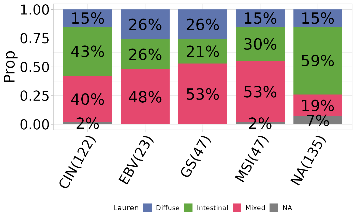
Create a Percent Bar Plot — percent_bar

Generates a bar plot visualizing the percentage distribution of a variable grouped by another variable.

Usage

percent_bar_plot(
  input,
  x,
  y,
  subset.x = NULL,
  color = NULL,
  palette = NULL,
  title = NULL,
  axis_angle = 0,
  coord_flip = FALSE,
  add_Freq = TRUE,
  Freq = "Proportion",
  size_freq = 8,
  legend.size = 0.5,
  legend.size.text = 10,
  add_sum = TRUE,
  print_result = TRUE,
  round.num = 2
)

Arguments

input: Input data frame.
x: Name of the x-axis variable.
y: Name of the y-axis (grouping) variable.
subset.x: Optional subset of x-axis values.
color: Optional color palette.
palette: Optional palette type.
title: Optional plot title.
axis_angle: Angle for axis labels (0-90). Default is 0.
coord_flip: Logical to flip coordinates. Default is FALSE.
add_Freq: Logical to add frequency count. Default is TRUE.
Freq: Name of frequency column.
size_freq: Size of frequency labels. Default is 8.
legend.size: Size of legend. Default is 0.5.
legend.size.text: Size of legend text. Default is 10.
add_sum: Logical to add sum to x-axis labels. Default is TRUE.
print_result: Logical to print result data frame. Default is TRUE.
round.num: Decimal places for proportion. Default is 2.

Value

A ggplot object.

Author

Dongqiang Zeng

Examples

# Simulate data
set.seed(123)
sim_data <- data.frame(
  Subtype = sample(c("EBV", "GS", "MSI", "CIN"), 100, replace = TRUE),
  Lauren = sample(c("Diffuse", "Intestinal", "Mixed"), 100, replace = TRUE)
)

# Create percent bar plot
p <- percent_bar_plot(
  input = sim_data, x = "Subtype", y = "Lauren",
  axis_angle = 60
)
#> # A tibble: 12 × 5
#> # Groups:   Subtype [4]
#>    Subtype Lauren      Freq  Prop count
#>    <chr>   <chr>      <dbl> <dbl> <dbl>
#>  1 CIN     Diffuse        6  0.35    17
#>  2 CIN     Intestinal     7  0.41    17
#>  3 CIN     Mixed          4  0.24    17
#>  4 EBV     Diffuse        5  0.18    28
#>  5 EBV     Intestinal    10  0.36    28
#>  6 EBV     Mixed         13  0.46    28
#>  7 GS      Diffuse        6  0.23    26
#>  8 GS      Intestinal    11  0.42    26
#>  9 GS      Mixed          9  0.35    26
#> 10 MSI     Diffuse        9  0.31    29
#> 11 MSI     Intestinal    11  0.38    29
#> 12 MSI     Mixed          9  0.31    29
#> ℹ Available categories: box, continue2, continue, random, heatmap, heatmap3, tidyheatmap
#> ℹ Random palettes: 1 (palette1), 2 (palette2), 3 (palette3), 4 (palette4)
#> '#5f75ae', '#64a841', '#e5486e', '#de8e06', '#b5aa0f', '#7ba39d', '#b15928', '#6a3d9a', '#cab2d6', '#374E55FF', '#80796BFF', '#e31a1c', '#fb9a99', '#1f78b4', '#a6cee3', '#008280FF', '#8F7700FF', '#A20056FF', '#fdbf6f', '#E78AC3', '#b2df8a', '#CD534CFF', '#008B45FF', '#67001F', '#00A087FF', '#A73030FF', '#386CB0', '#F0027F', '#666666', '#EFC000FF', '#003C67FF', '#7AA6DCFF', '#8F7700FF', '#33a02c', '#66C2A5', '#A6D854', '#E5C494', '#6A3D9A', '#374E55FF', '#DF8F44FF', '#8DA0CB', '#80796BFF', '#FFFF99', '#E78AC3', '#7FC97F', '#3B3B3BFF', '#B24745FF', '#3B4992FF', '#631879FF', '#7AA6DCFF', '#7ba39d', '#b15928', '#00A1D5FF', '#a6a6a6', '#386CB0', '#F0027F', '#1B9E77', '#7570B3', '#67001F', '#4DBBD5FF', '#F39B7FFF', '#7FC97F', '#BEAED4', '#224444', '#DF8F44FF', '#B24745FF', '#3B4992FF', '#631879FF', '#7AA6DCFF', '#003C67FF', '#8F7700FF', '#3B3B3BFF', '#984EA3', '#a6a6a6', '#8DA0CB', '#E78AC3', '#FFD92F', '#8DD3C7', '#1F78B4', '#66A61E', '#D62728FF', '#9467BDFF', '#8C564BFF', '#E377C2FF', '#7F7F7FFF', '#17BECFFF', '#FB9A99', '#FDBF6F', '#33adff', '#439373', '#92C5DE', '#CAB2D6'

if (!is.null(p)) print(p)