Figures and export

Start from saved results when your numbers already exist. The original figures below are retained unchanged from earlier examples; they are not outputs of the Book’s small synthetic installation check.

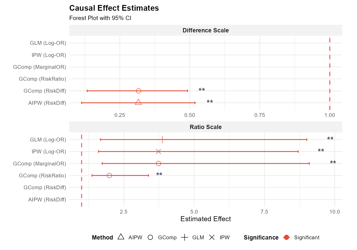
Forest plot

Read the estimate, its interval and its own reference scale. Compare compatible contrasts; a risk difference and an OR cannot share one numerical interpretation.

Original forest plot

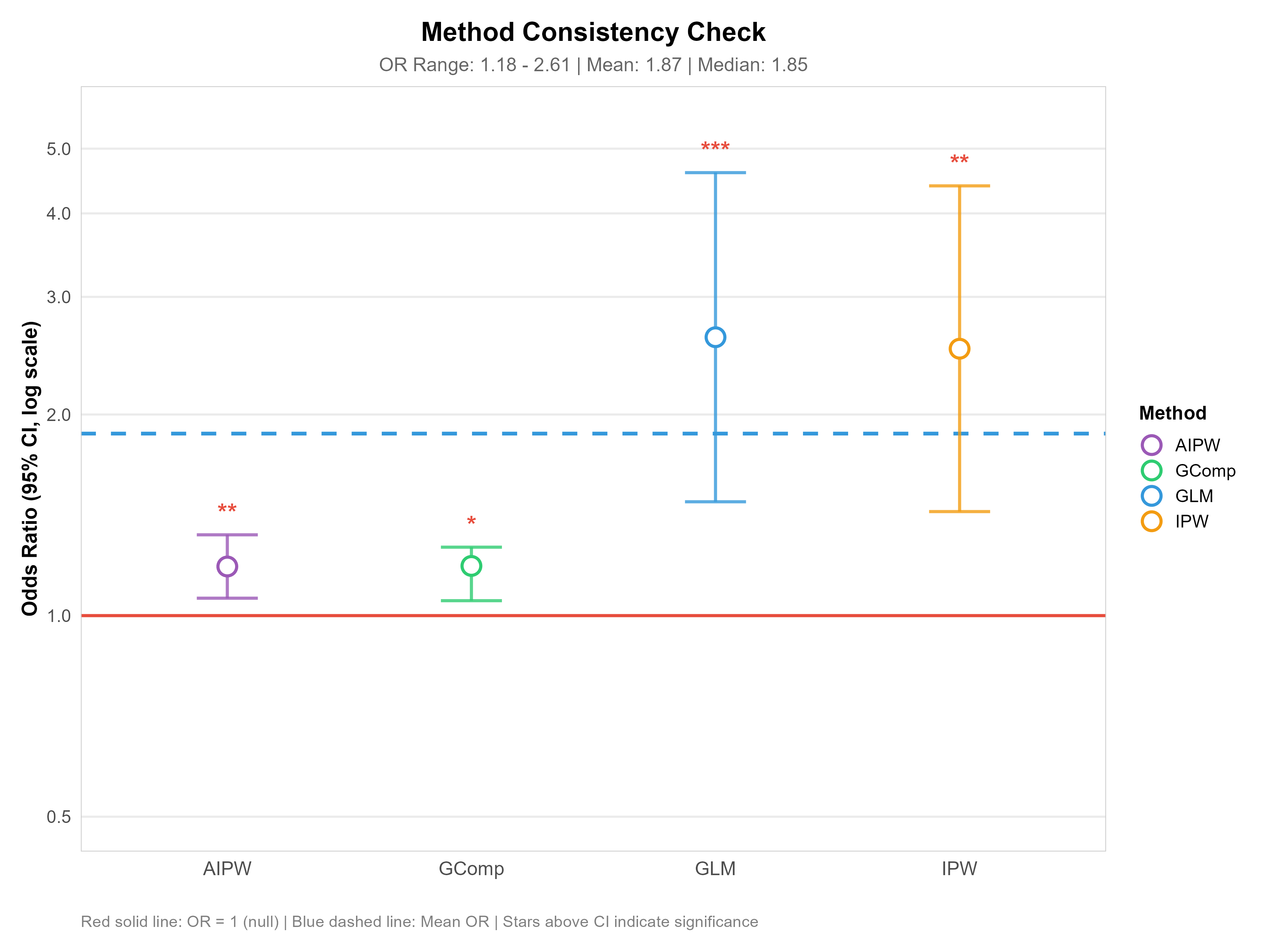
Method consistency

Look for agreement and disagreement across methods. Shared assumptions or bias can produce agreement, so this plot does not independently establish causality.

Original method consistency plot

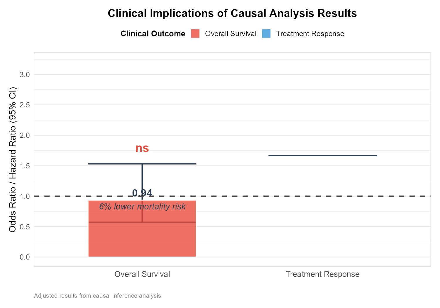
Clinical summary

Response and OS describe different endpoints. Keep odds ratios, hazard ratios and absolute survival contrasts distinct.

Original clinical implications plot

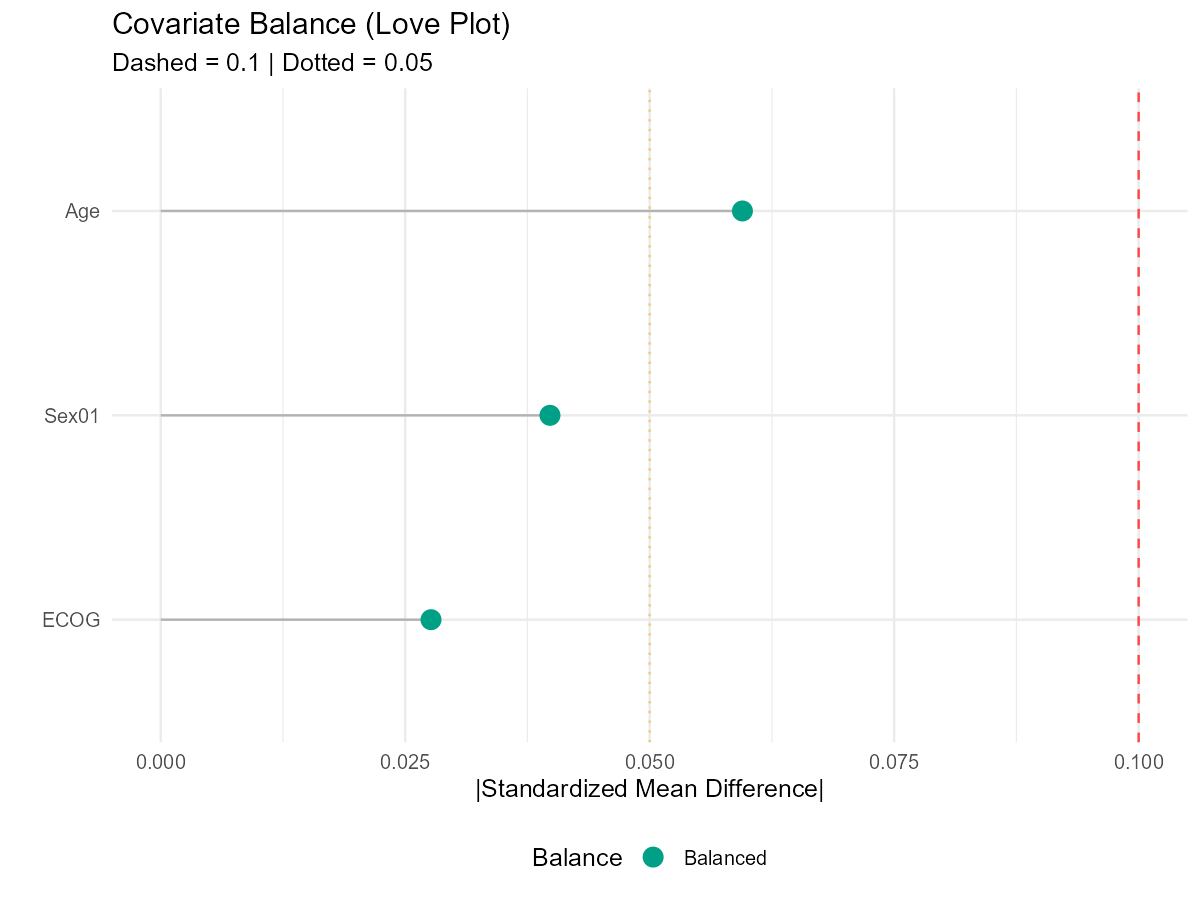
Covariate balance

Inspect standardized differences before and after adjustment. Balance on measured covariates does not prove exchangeability or absence of hidden confounding.

Original Love plot

Advanced R plotting

These direct R functions are useful for an existing workflow object res:

iobr_causal_plot(res, type = "forest")
iobr_causal_visual_report(res, output_dir = "figures",
                         formats = c("png", "pdf", "svg"))

For a pathway-first object, use iobr_causal_pathway_first_visual_report() for the route-specific overview. Read the help for functions that may compute curves; the shared saved-number plot operation has a separate no-fit contract.

Use PNG for a quick preview, PDF for layout and SVG for editable vector output. Keep the source tables, full rows and provenance with the figures. Historical numeric context is in the original examples appendix.