Chapter 6 Signature Score and Relevant phenotypes
6.2 Downloading data for example
Obtaining data set from GEO Gastric cancer: GSE62254 using GEOquery R package.
if (!requireNamespace("GEOquery", quietly = TRUE)) BiocManager::install("GEOquery")
library("GEOquery")
# NOTE: This process may take a few minutes which depends on the internet connection speed. Please wait for its completion.
eset_geo <- getGEO(GEO = "GSE62254", getGPL = F, destdir = "./")
eset <- eset_geo[[1]]
eset <- exprs(eset)
eset[1:5, 1:5]
## GSM1523727 GSM1523728 GSM1523729 GSM1523744 GSM1523745
## 1007_s_at 3.2176645 3.0624323 3.0279131 2.921683 2.8456013
## 1053_at 2.4050109 2.4394879 2.2442708 2.345916 2.4328582
## 117_at 1.4933412 1.8067380 1.5959665 1.839822 1.8326058
## 121_at 2.1965561 2.2812181 2.1865556 2.258599 2.1874363
## 1255_g_at 0.8698382 0.9502466 0.8125414 1.012860 0.94419936.3 Gene Annotation
Annotation of genes in the expression matrix and removal of duplicate genes.
# Load the annotation file `anno_hug133plus2` in IOBR.
anno_hug133plus2 <- load_data("anno_hug133plus2")
head(anno_hug133plus2)
## # A tibble: 6 × 2
## probe_id symbol
## <fct> <fct>
## 1 1007_s_at MIR4640
## 2 1053_at RFC2
## 3 117_at HSPA6
## 4 121_at PAX8
## 5 1255_g_at GUCA1A
## 6 1294_at MIR5193# Conduct gene annotation using `anno_hug133plus2` file; If identical gene symbols exists, these genes would be ordered by the mean expression levels. The gene symbol with highest mean expression level is selected and remove others.
eset <- anno_eset(
eset = eset,
annotation = anno_hug133plus2,
symbol = "symbol",
probe = "probe_id",
method = "mean"
)
eset[1:5, 1:3]## GSM1523727 GSM1523728 GSM1523729
## SH3KBP1 4.327974 4.316195 4.351425
## RPL41 4.246149 4.246808 4.257940
## EEF1A1 4.293762 4.291038 4.262199
## COX2 4.250288 4.283714 4.270508
## LOC101928826 4.219303 4.219670 4.2132526.4 Estimation of signatures
signature_collection <- load_data("signature_collection")
sig_tme <- calculate_sig_score(
  pdata = NULL,
  eset = eset,
  signature = signature_collection,
  method = "pca",
  mini_gene_count = 2
)

sig_tme <- t(column_to_rownames(sig_tme, var = "ID"))
sig_tme[1:5, 1:3]
## GSM1523727 GSM1523728 GSM1523729
## CD_8_T_effector -2.5513794 0.7789141 -2.1770675
## DDR -0.8747614 0.7425162 -1.3272054
## APM 1.1098368 2.1988688 -0.9516419
## Immune_Checkpoint -2.3701787 0.9455120 -1.4844104
## CellCycle_Reg 0.1063358 0.7583302 -0.36497956.5 Combining score data and phenotype data
##            ID ProjectID  Technology       platform Gender Age RFS_time
## 71 GSM1523727  GSE62254 Affymetrix  HG-U133_Plus_2      M  67     3.97
## 72 GSM1523728  GSE62254 Affymetrix  HG-U133_Plus_2      F  68     4.03
## 73 GSM1523729  GSE62254 Affymetrix  HG-U133_Plus_2      F  42    74.97
## 74 GSM1523744  GSE62254 Affymetrix  HG-U133_Plus_2      M  69    89.77
## 75 GSM1523745  GSE62254 Affymetrix  HG-U133_Plus_2      M  68    84.60
## 76 GSM1523746  GSE62254 Affymetrix  HG-U133_Plus_2      M  56     5.77
##    RFS_status OS_time OS_status     Lauren Differtiation AJCC_Stage_confuse
## 71         NA   88.73         0 Intestinal            MD                  2
## 72         NA   88.23         0 Intestinal            PD                  2
## 73          0   88.23         0    Diffuse            PD                  2
## 74          0  105.70         0    Diffuse            PD                  2
## 75          0  105.53         0    Diffuse            PD                  3
## 76          1   25.50         1      Mixed            PD                  2
##    T_stage N_stage M_stage Lymph_node_examined Positive_lymph_nodes
## 71       2       1       0                  20                    3
## 72       2       1       0                  40                    1
## 73       2       1       0                  21                    1
## 74       2       1       0                  24                    3
## 75       3       2       0                  52                   11
## 76       2       1       0                  22                    5
##    Revisedlocation MSI EBV Hpylori   Subtype TP53mutated B.cells.naive
## 71            Body   1   0      NA       MSI           0   0.006611704
## 72            Body   1  NA      NA       MSI           0   0.000000000
## 73          Antrum   0   0       0 MSS/TP53+           1   0.003306927
## 74          Antrum   1   0       1       MSI           0   0.000000000
## 75          Antrum   0   0      NA MSS/TP53-           0   0.000000000
## 76          Antrum   0   0       0 MSS/TP53-           0   0.013619480
##    B.cells.memory Plasma.cells T.cells.CD8 T.cells.CD4.naive
## 71    0.014570868   0.17555729  0.05712737                 0
## 72    0.036202099   0.08523233  0.05336971                 0
## 73    0.020935673   0.10489546  0.00000000                 0
## 74    0.072648177   0.08755997  0.03465107                 0
## 75    0.009798381   0.12251030  0.00000000                 0
## 76    0.012784581   0.15602714  0.00000000                 0
##    T.cells.CD4.memory.resting T.cells.CD4.memory.activated
## 71                  0.1439895                  0.025159835
## 72                  0.1250515                  0.049617381
## 73                  0.1849220                  0.008407981
## 74                  0.1396439                  0.055268600
## 75                  0.1916398                  0.036578672
## 76                  0.1905921                  0.008992440
##    T.cells.follicular.helper T.cells.regulatory..Tregs. T.cells.gamma.delta
## 71                0.02453957                          0          0.00000000
## 72                0.05318251                          0          0.00000000
## 73                0.05098080                          0          0.03714459
## 74                0.07825130                          0          0.00000000
## 75                0.02223859                          0          0.02657259
## 76                0.04740728                          0          0.04283296
##    NK.cells.resting NK.cells.activated Monocytes Macrophages.M0 Macrophages.M1
## 71      0.000000000        0.049325657         0     0.03865693     0.06910287
## 72      0.000000000        0.081481924         0     0.07370723     0.08016443
## 73      0.000000000        0.025252673         0     0.00000000     0.06161940
## 74      0.000000000        0.016121853         0     0.08866391     0.08173804
## 75      0.001738259        0.006267907         0     0.15255902     0.07161270
## 76      0.000000000        0.052117471         0     0.10298038     0.03246627
##    Macrophages.M2 Dendritic.cells.resting Dendritic.cells.activated
## 71      0.1829208               0.0000000               0.022904531
## 72      0.1320919               0.0000000               0.060491149
## 73      0.1170839               0.1171129               0.032385282
## 74      0.1441202               0.0000000               0.060937005
## 75      0.1919279               0.0000000               0.006087801
## 76      0.1093805               0.0000000               0.023914527
##    Mast.cells.resting Mast.cells.activated Eosinophils Neutrophils.x P.value
## 71        0.069286038          0.000000000 0.006315889    0.11393115       0
## 72        0.003322764          0.005197745 0.056141443    0.10474585       0
## 73        0.052571970          0.000000000 0.104493538    0.07888690       0
## 74        0.012494201          0.006833953 0.050435095    0.07063272       0
## 75        0.000000000          0.033928747 0.017164438    0.10937487       0
## 76        0.014373257          0.002764802 0.115772442    0.07397439       0
##    Pearson.Correlation      RMSE    T.cells CD8.T.cells Cytotoxic.lymphocytes
## 71           0.3359926 0.9415173 -0.9275804   0.8492914            -1.1005262
## 72           0.4793134 0.8827802 -0.5306279  -0.2017907             0.1858499
## 73           0.3638005 0.9308186 -0.9566316   0.2411951            -0.8800338
## 74           0.3569989 0.9332100 -1.0464552  -0.5771205            -0.5619472
## 75           0.4226987 0.9062522 -0.6796120   0.6670229            -0.3361456
## 76           0.4113346 0.9112588 -0.6978480  -1.1110102            -0.7631710
##        NK.cells   B.lineage Monocytic.lineage Myeloid.dendritic.cells
## 71 -0.083623737 -0.54974243       -1.40389061              -0.7589211
## 72  0.156167025 -0.33750363       -0.03696397              -0.6393975
## 73  0.003538847  0.01597566       -0.67105808               0.7452174
## 74 -0.010774923 -0.56740438        0.06877240              -0.2511140
## 75 -0.028429092 -0.73180429        0.21574792              -0.1165082
## 76  0.466964699  0.15583392       -0.97524359              -0.7448360
##    Neutrophils.y Endothelial.cells Fibroblasts StromalScore ImmuneScore
## 71    -0.9527759       -1.42753593 -1.22754105   -1.8047694  -1.3347047
## 72     0.5640500       -0.17320689  0.41586717    0.1825225   0.1950604
## 73    -0.3415288       -0.25784297  0.04110246   -0.1863425  -0.4960305
## 74    -1.2984378       -1.05394707  0.00743277   -0.2731398  -0.7950682
## 75     0.4227674        0.03025664  0.32245183    0.3165798  -0.2416774
## 76    -0.4411653       -0.29582293 -0.68833740   -0.9119449  -0.8475150
##    ESTIMATEScore TumorPurity ProjectID2   TMEscoreA    TMEscoreB    TMEscore
## 71   -1.70632719   1.1687573   GSE62254 -1.06110812 -1.270222413  0.60585688
## 72    0.20292720          NA   GSE62254  1.14698153 -0.333585646  0.73717229
## 73   -0.35721073  -1.3859061   GSE62254 -0.89026369 -0.007906066 -0.35452887
## 74   -0.55795758  -0.9855180   GSE62254 -0.01116022 -0.984841623  0.79880007
## 75    0.05885805          NA   GSE62254 -0.27102383 -0.017592784 -0.09554256
## 76   -0.94967710  -0.2162267   GSE62254 -0.94526260  0.161818627 -0.51527214
##    TMEscore_binary
## 71             Low
## 72            High
## 73             Low
## 74            High
## 75             Low
## 76 Low6.6 Identifying features associated with survival
res <- batch_surv(
  pdata = input,
  time = "OS_time",
  status = "OS_status",
  variable = colnames(input)[69:ncol(input)]
)
head(res)
## # A tibble: 6 × 5
## P HR CI_low_0.95 CI_up_0.95 ID
## <dbl> <dbl> <dbl> <dbl> <chr>
## 1 1.00e-10 0.579 0.490 0.683 Folate_biosynthesis
## 2 1.32e- 9 0.640 0.554 0.739 TMEscore_CIR
## 3 3.24e- 9 1.52 1.32 1.74 Glycogen_Biosynthesis
## 4 6.33e- 9 1.55 1.34 1.80 Pan_F_TBRs
## 5 7.17e- 9 1.52 1.32 1.75 TMEscoreB_CIR
## 6 8.08e- 9 0.638 0.547 0.743 TMEscore_plusUse forest plots sig_forest to show the most relevant variables to overall survival
6.7 Visulization using heatmap
Relationship between Signatures and molecular typing.
Heatmap visualisation using IOBR’s sig_heatmap
p2 <- sig_heatmap(
  input = input,
  features = res$ID[1:20],
  group = "Subtype",
  palette_group = "jama",
  palette = 6,
  path = "result"
)
## Warning: `when()` was deprecated in purrr 1.0.0.
## ℹ Please use `if` instead.
## ℹ The deprecated feature was likely used in the tidyHeatmap package.
## Please report the issue at
## <https://github.com/stemangiola/tidyHeatmap/issues>.
## This warning is displayed once per session.
## Call `lifecycle::last_lifecycle_warnings()` to see where this warning was
## generated.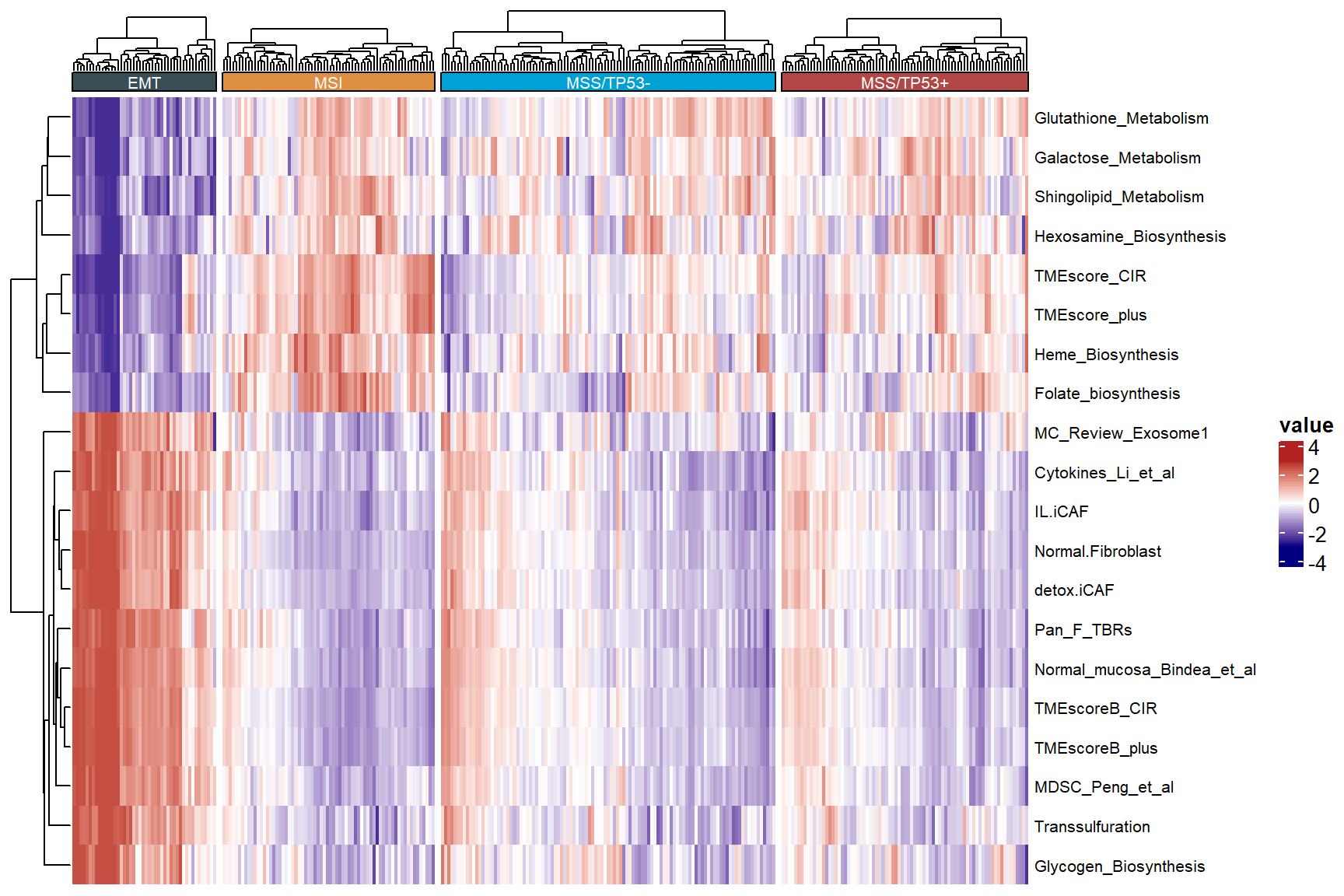
6.8 Focus on target signatures
p1 <- sig_box(
  data = input,
  signature = "Glycogen_Biosynthesis",
  variable = "Subtype",
  jitter = FALSE,
  cols = NULL,
  palette = "jama",
  show_pairwise_p = TRUE,
  size_of_pvalue = 5,
  hjust = 1,
  angle_x_text = 60,
  size_of_font = 8
)
## # A tibble: 6 × 8
## .y. group1 group2 p p.adj p.format p.signif method
## <chr> <chr> <chr> <dbl> <dbl> <chr> <chr> <chr>
## 1 signature EMT MSI 5.39e-15 3.20e-14 5.4e-15 **** Wilcoxon
## 2 signature EMT MSS/TP53- 5.53e-13 2.8 e-12 5.5e-13 **** Wilcoxon
## 3 signature MSI MSS/TP53- 1.14e- 3 3.4 e- 3 0.0011 ** Wilcoxon
## 4 signature EMT MSS/TP53+ 1.90e-12 7.6 e-12 1.9e-12 **** Wilcoxon
## 5 signature MSI MSS/TP53+ 7.05e- 3 1.4 e- 2 0.0071 ** Wilcoxon
## 6 signature MSS/TP53- MSS/TP53+ 7.16e- 1 7.2 e- 1 0.7161 ns Wilcoxonp2 <- sig_box(
data = input,
signature = "Pan_F_TBRs",
variable = "Subtype",
jitter = FALSE,
cols = NULL,
palette = "jama",
show_pairwise_p = TRUE,
angle_x_text = 60,
hjust = 1,
size_of_pvalue = 5,
size_of_font = 8
)## # A tibble: 6 × 8
## .y. group1 group2 p p.adj p.format p.signif method
## <chr> <chr> <chr> <dbl> <dbl> <chr> <chr> <chr>
## 1 signature EMT MSI 7.98e-17 3.20e-16 <2e-16 **** Wilcoxon
## 2 signature EMT MSS/TP53- 1.70e-17 1 e-16 <2e-16 **** Wilcoxon
## 3 signature MSI MSS/TP53- 1.32e- 2 4 e- 2 0.013 * Wilcoxon
## 4 signature EMT MSS/TP53+ 2.57e-17 1.3 e-16 <2e-16 **** Wilcoxon
## 5 signature MSI MSS/TP53+ 6.99e- 2 1.4 e- 1 0.070 ns Wilcoxon
## 6 signature MSS/TP53- MSS/TP53+ 4.02e- 1 4 e- 1 0.402 ns Wilcoxonp3 <- sig_box(
data = input,
signature = "Immune_Checkpoint",
variable = "Subtype",
jitter = FALSE,
cols = NULL,
palette = "jama",
show_pairwise_p = TRUE,
angle_x_text = 60,
hjust = 1,
size_of_pvalue = 5,
size_of_font = 8
)## # A tibble: 6 × 8
## .y. group1 group2 p p.adj p.format p.signif method
## <chr> <chr> <chr> <dbl> <dbl> <chr> <chr> <chr>
## 1 signature EMT MSI 2.20e- 2 0.044 0.0220 * Wilcoxon
## 2 signature EMT MSS/TP53- 2.11e- 3 0.0085 0.0021 ** Wilcoxon
## 3 signature MSI MSS/TP53- 9.13e-10 0.0000000055 9.1e-10 **** Wilcoxon
## 4 signature EMT MSS/TP53+ 4.03e- 1 0.4 0.4026 ns Wilcoxon
## 5 signature MSI MSS/TP53+ 5.03e- 4 0.0025 0.0005 *** Wilcoxon
## 6 signature MSS/TP53- MSS/TP53+ 4.82e- 3 0.014 0.0048 ** Wilcoxon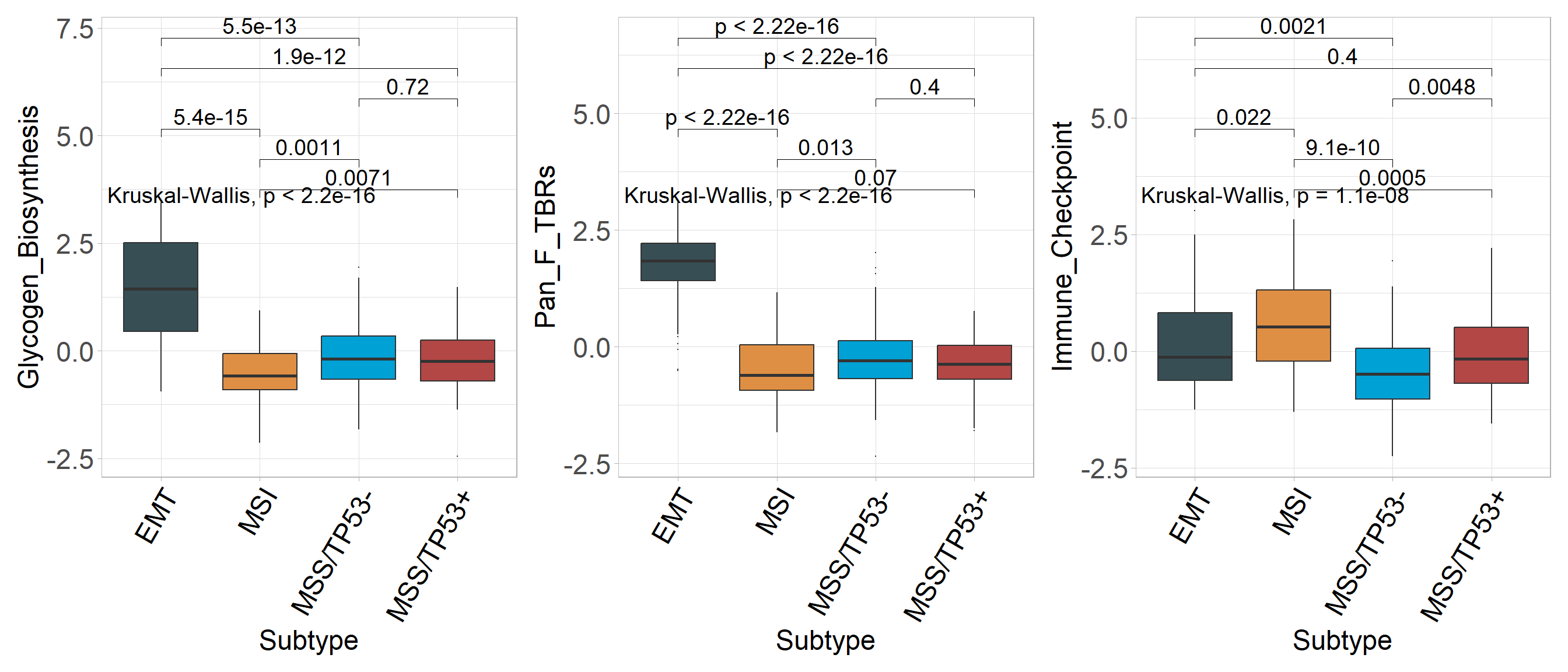
6.9 Survival analysis and visulization
6.9.1 Kaplan-Meier plot
Displaying the outcomes of survival analyses using Kaplan-Meier plot. Multiple stratifications of the signature were used to judge the efficacy of this metric in predicting patient survival.
res <- sig_surv_plot(
  input_pdata = input,
  signature = "Glycogen_Biosynthesis",
  cols = NULL,
  palette = "jama",
  project = "ACRG",
  time = "OS_time",
  status = "OS_status",
  time_type = "month",
  save_path = "result"
)
res$plots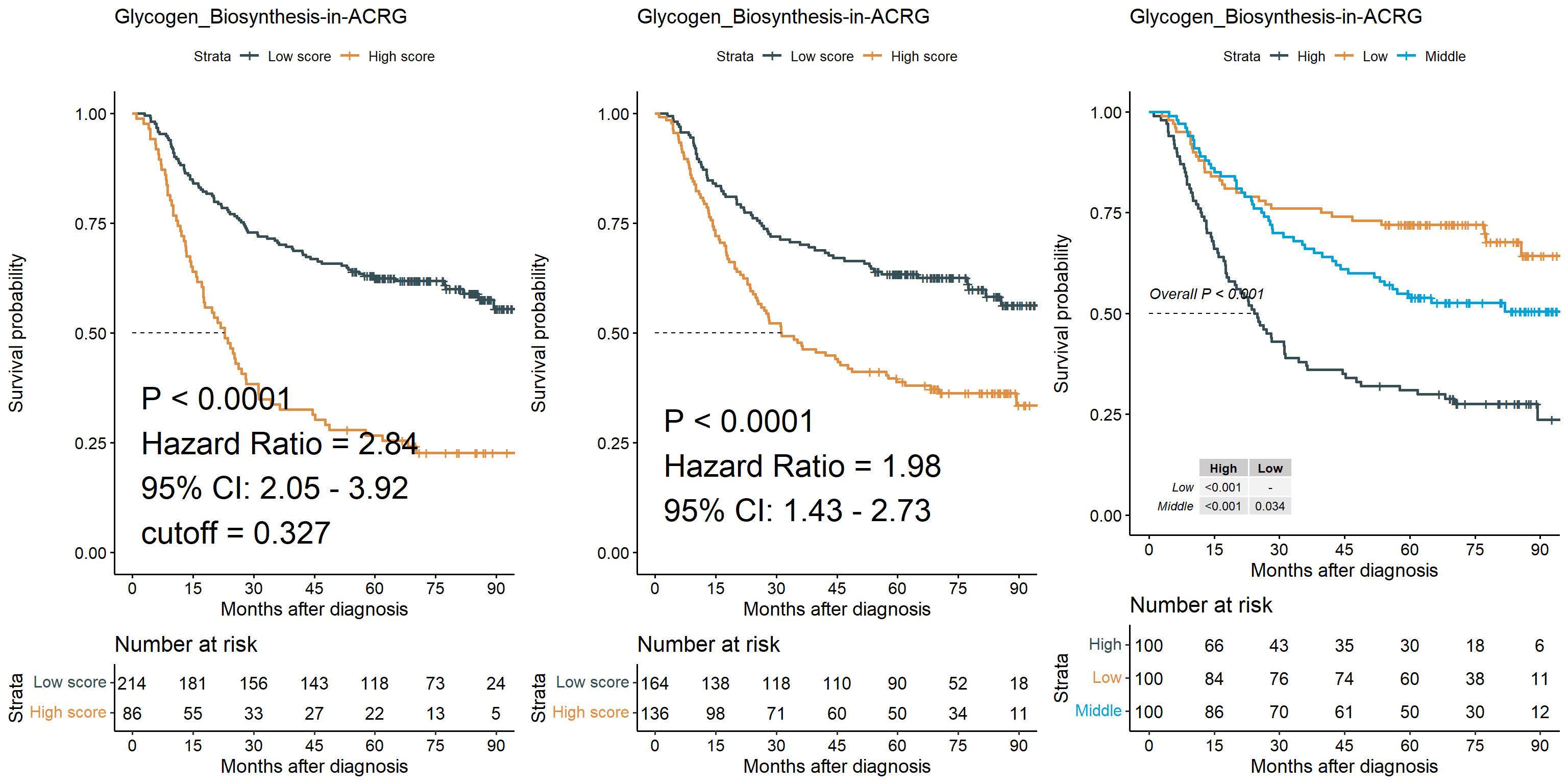
6.9.2 Time-Dependent ROC curve
p1 <- roc_time(
  input = input,
  vars = "Glycogen_Biosynthesis",
  time = "OS_time",
  status = "OS_status",
  time_point = c(12, 24, 36),
  time_type = "month",
  palette = "jama",
  cols = "normal",
  seed = 1234,
  show_col = FALSE,
  path = "result",
  main = "OS",
  index = 1,
  fig.type = "pdf",
  width = 5,
  height = 5.2
)

p2 <- roc_time(
  input = input,
  vars = "Glycogen_Biosynthesis",
  time = "RFS_time",
  status = "RFS_status",
  time_point = c(12, 24, 36),
  time_type = "month",
  palette = "jama",
  cols = "normal",
  seed = 1234,
  show_col = FALSE,
  path = "result",
  main = "OS",
  index = 1,
  fig.type = "pdf",
  width = 5,
  height = 5.2
)
p1 | p2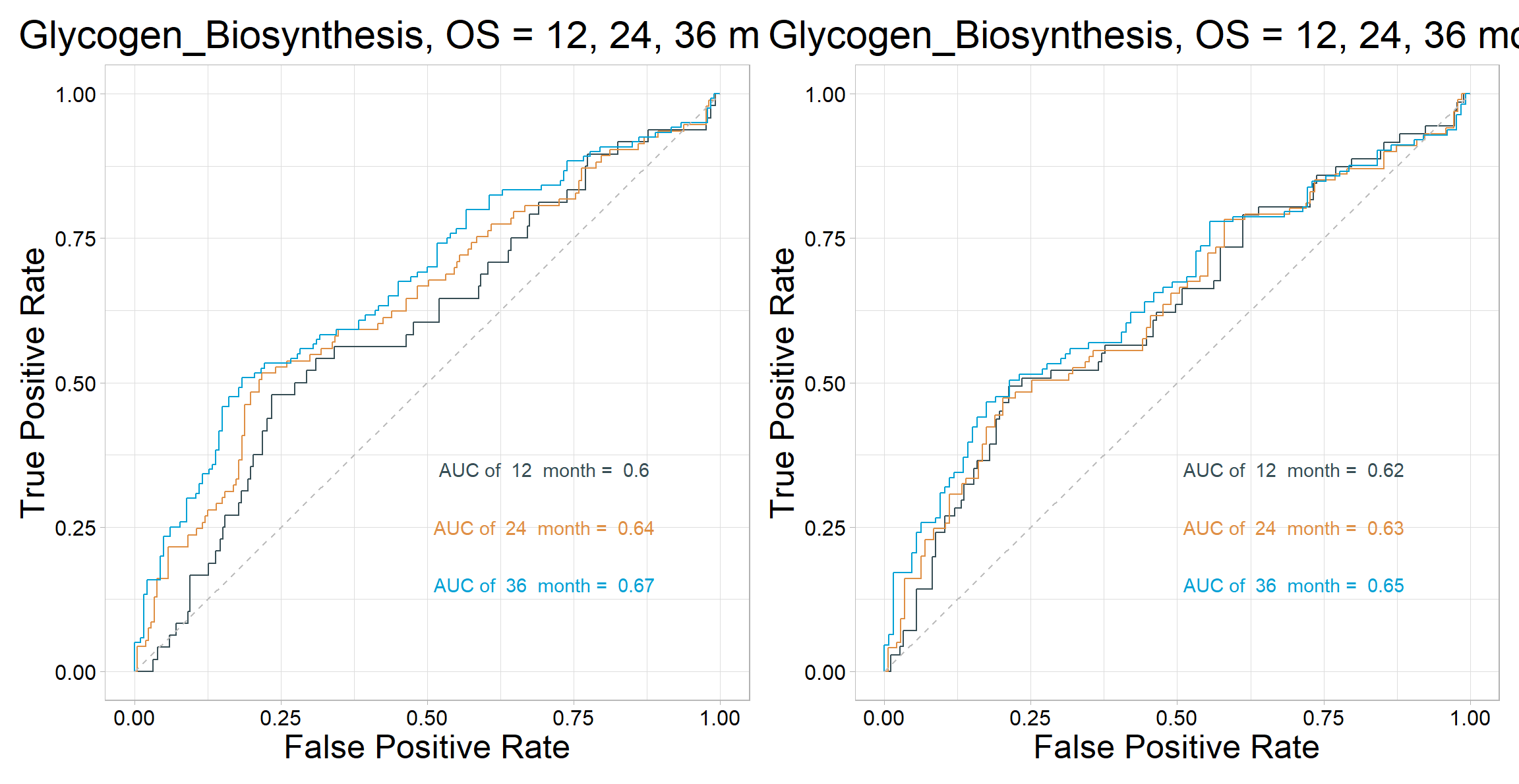
6.10 Batch correlation analysis
6.10.1 Finding continuity variables associated with signatures
Identifying genes or signatures related to the target signatures
6.10.1.1 Correlation between two variables
res <- batch_cor(data = input, target = "Glycogen_Biosynthesis", feature = colnames(input)[69:ncol(input)])## ℹ Computing spearman correlation for 314 features## ✔ Correlation analysis complete## # A tibble: 6 × 6
## sig_names p.value statistic p.adj log10pvalue stars
## <chr> <dbl> <dbl> <dbl> <dbl> <fct>
## 1 TMEscoreB_CIR 8.89e-42 0.678 2.79e-39 41.1 ****
## 2 Glycine__Serine_and_Threonine_M… 7.49e-40 -0.666 1.18e-37 39.1 ****
## 3 Ether_Lipid_Metabolism 3.84e-39 0.662 4.02e-37 38.4 ****
## 4 MDSC_Peng_et_al 1.13e-38 0.659 8.88e-37 37.9 ****
## 5 Glycerophospholipid_Metabolism 8.72e-38 -0.653 5.47e-36 37.1 ****
## 6 TIP_Release_of_cancer_cell_anti… 2.32e-37 -0.650 1.21e-35 36.6 ****p1 <- get_cor(
eset = sig_tme, pdata = pdata_acrg, is.matrix = TRUE, var1 = "Glycogen_Biosynthesis",
var2 = "TMEscore_CIR", subtype = "Subtype", palette = "aaas", path = "result"
)##
## Spearman's rank correlation rho
##
## data: data[[var1]] and data[[var2]]
## S = 7282858, p-value < 2.2e-16
## alternative hypothesis: true rho is not equal to 0
## sample estimates:
## rho
## -0.6184309p2 <- get_cor(
eset = sig_tme, pdata = pdata_acrg, is.matrix = TRUE, var1 = "Glycogen_Biosynthesis",
var2 = "TGFβ_myCAF", subtype = "Subtype", palette = "aaas", path = "result"
)##
## Spearman's rank correlation rho
##
## data: data[[var1]] and data[[var2]]
## S = 2430178, p-value < 2.2e-16
## alternative hypothesis: true rho is not equal to 0
## sample estimates:
## rho
## 0.4599544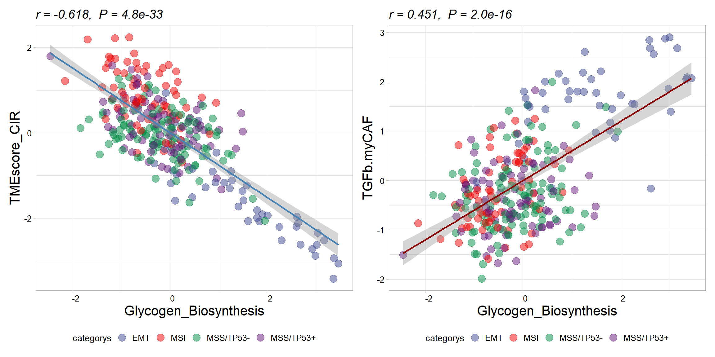
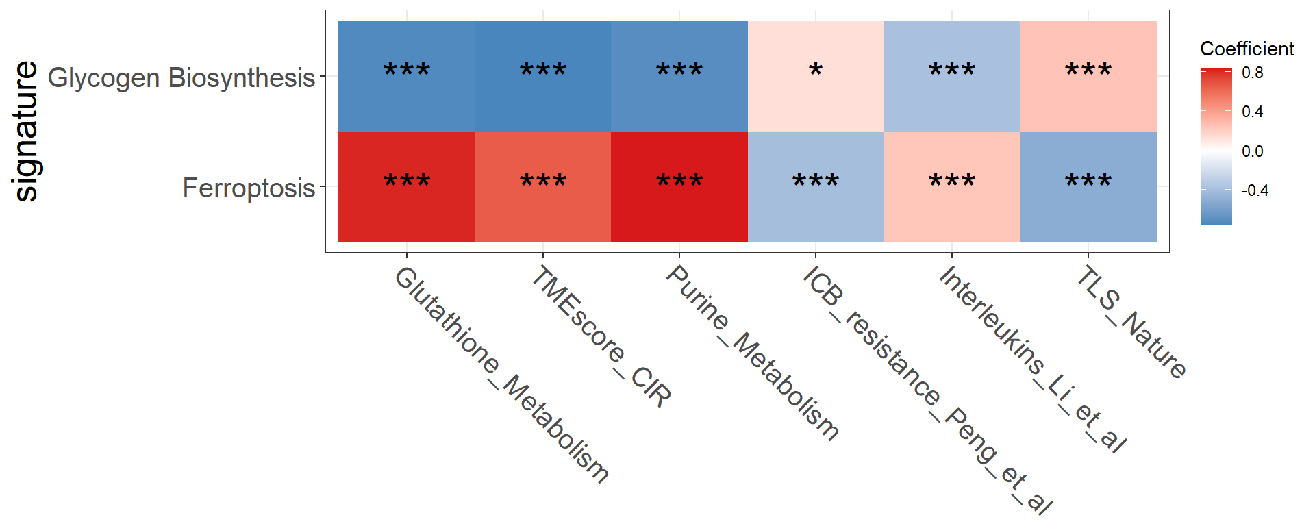
6.10.1.2 Demonstrate correlation between multiple variables
Visualisation via correlation matrix
feas1 <- c("Glycogen_Biosynthesis", "Ferroptosis")
feas2 <- c("Glutathione_Metabolism", "TMEscore_CIR", "Purine_Metabolism", "ICB_resistance_Peng_et_al", "Interleukins_Li_et_al", "TLS_Nature")
p <- get_cor_matrix(
  data = input,
  feas1 = feas2,
  feas2 = feas1,
  method = "pearson",
  font.size.star = 8,
  font.size = 15,
  fill_by_cor = FALSE,
  round.num = 1,
  path = "result"
)
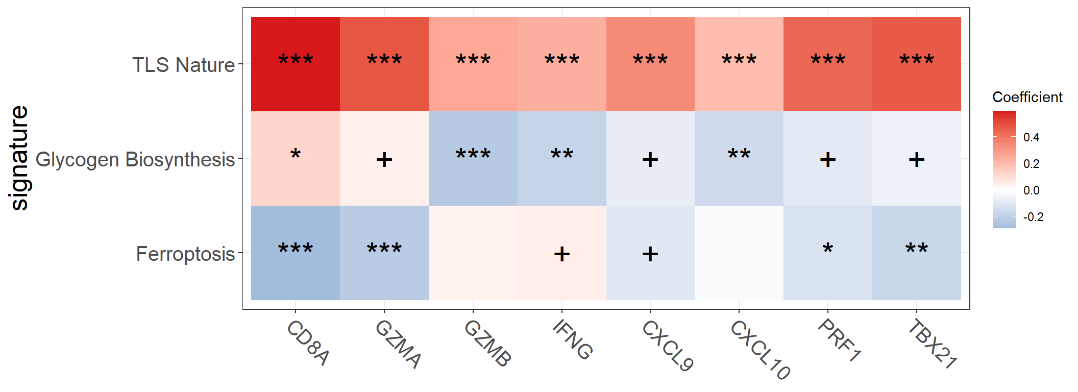
Demonstrate the correlation between signatures and genes
input2 <- combine_pd_eset(eset = eset, pdata = input[, c("ID", "Glycogen_Biosynthesis", "TLS_Nature", "Ferroptosis")])
feas1 <- c("Glycogen_Biosynthesis", "TLS_Nature", "Ferroptosis")
feas2 <- signature_collection$CD_8_T_effector
feas2
## [1] "CD8A" "GZMA" "GZMB" "IFNG" "CXCL9" "CXCL10" "PRF1" "TBX21"p <- get_cor_matrix(
data = input2,
feas1 = feas2,
feas2 = feas1,
method = "pearson",
scale = T,
font.size.star = 8,
font.size = 15,
fill_by_cor = FALSE,
round.num = 1,
path = "result"
)
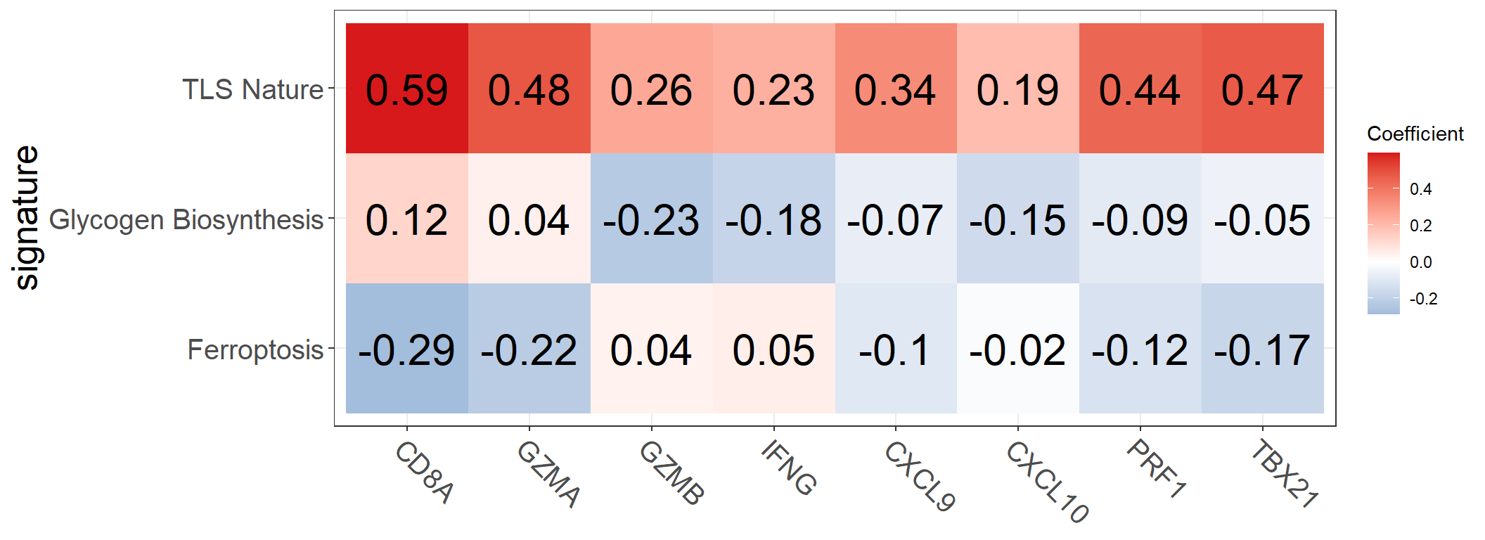
Users can customize the image using parameters.
p <- get_cor_matrix(
  data = input2,
  feas1 = feas2,
  feas2 = feas1,
  method = "pearson",
  scale = T,
  font.size.star = 8,
  font.size = 15,
  fill_by_cor = TRUE,
  round.num = 2,
  path = "result"
)
6.10.2 Identifying Category Variables Linked to Signatures
6.10.2.1 For binary variable
res <- batch_wilcoxon(data = input, target = "TMEscore_binary", feature = colnames(input)[69:ncol(input)])
head(res)
## # A tibble: 6 × 8
## sig_names p.value High Low statistic p.adj log10pvalue stars
## <chr> <dbl> <dbl> <dbl> <dbl> <dbl> <dbl> <fct>
## 1 TMEscore_CIR 4.44e-37 1.17 -0.365 1.54 1.40e-34 36.4 ****
## 2 TMEscore_plus 3.97e-34 1.23 -0.380 1.61 6.25e-32 33.4 ****
## 3 TMEscoreA_plus 1.68e-25 1.18 -0.359 1.54 1.77e-23 24.8 ****
## 4 TMEscoreB_CIR 5.59e-24 -0.881 0.279 -1.16 4.13e-22 23.3 ****
## 5 ADP_Ribosylation 6.56e-24 1.06 -0.329 1.39 4.13e-22 23.2 ****
## 6 TMEscoreA_CIR 1.02e-22 1.11 -0.337 1.45 4.68e-21 22.0 ****p1 <- sig_box(
data = input,
signature = res$sig_names[1],
variable = "TMEscore_binary",
jitter = FALSE,
cols = NULL,
palette = "jco",
show_pairwise_p = TRUE,
size_of_pvalue = 5,
hjust = 1,
angle_x_text = 60,
size_of_font = 8
)## # A tibble: 1 × 8
## .y. group1 group2 p p.adj p.format p.signif method
## <chr> <chr> <chr> <dbl> <dbl> <chr> <chr> <chr>
## 1 signature High Low 4.44e-37 4.40e-37 <2e-16 **** Wilcoxonp2 <- sig_box(
data = input,
signature = res$sig_names[2],
variable = "TMEscore_binary",
jitter = FALSE,
cols = NULL,
palette = "jco",
show_pairwise_p = TRUE,
angle_x_text = 60,
hjust = 1,
size_of_pvalue = 5,
size_of_font = 8
)## # A tibble: 1 × 8
## .y. group1 group2 p p.adj p.format p.signif method
## <chr> <chr> <chr> <dbl> <dbl> <chr> <chr> <chr>
## 1 signature High Low 3.97e-34 4e-34 <2e-16 **** Wilcoxonp3 <- sig_box(
data = input,
signature = res$sig_names[3],
variable = "TMEscore_binary",
jitter = FALSE,
cols = NULL,
palette = "jco",
show_pairwise_p = TRUE,
angle_x_text = 60,
hjust = 1,
size_of_pvalue = 5,
size_of_font = 8
)## # A tibble: 1 × 8
## .y. group1 group2 p p.adj p.format p.signif method
## <chr> <chr> <chr> <dbl> <dbl> <chr> <chr> <chr>
## 1 signature High Low 1.68e-25 1.70e-25 <2e-16 **** Wilcoxon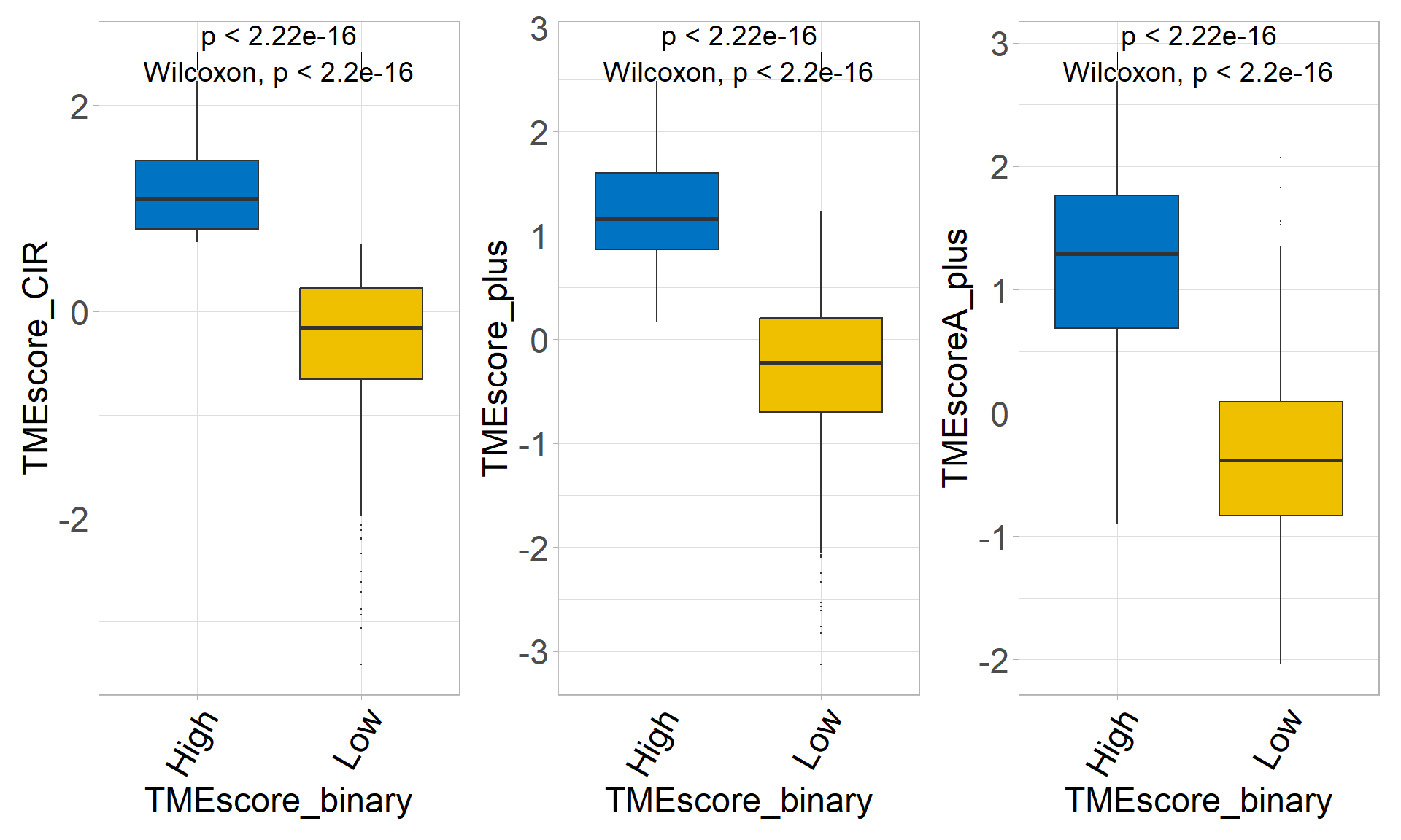
6.10.3 For multicategorical variables (>2 subgroups)
res <- batch_kruskal(data = input, group = "Subtype", feature = colnames(input)[69:ncol(input)])
head(res)
## # A tibble: 6 × 10
## sig_names p.value statistic EMT MSI `MSS/TP53+` `MSS/TP53-` p.adj
## <chr> <dbl> <dbl> <dbl> <dbl> <dbl> <dbl> <dbl>
## 1 TMEscore_CIR 1.35e-28 133. -1.36 1.000 0.305 0.0577 4.26e-26
## 2 Ether_Lipid_… 4.37e-27 126. 1.46 -0.830 -0.253 -0.375 5.71e-25
## 3 TMEscoreB_CIR 5.88e-27 125. 1.55 -0.829 -0.420 -0.303 5.71e-25
## 4 Inositol_Pho… 7.25e-27 125. 1.53 -0.808 -0.315 -0.408 5.71e-25
## 5 Selenocompou… 1.17e-26 124. -1.48 0.824 0.328 0.326 7.38e-25
## 6 Folate_biosy… 1.63e-26 123. -1.12 1.05 0.127 -0.0573 7.57e-25
## # ℹ 2 more variables: log10pvalue <dbl>, stars <fct>p1 <- sig_box(
data = input,
signature = res$sig_names[1],
variable = "Subtype",
jitter = FALSE,
cols = NULL,
palette = "jco",
show_pairwise_p = TRUE,
size_of_pvalue = 5,
hjust = 1,
angle_x_text = 60,
size_of_font = 8
)## # A tibble: 6 × 8
## .y. group1 group2 p p.adj p.format p.signif method
## <chr> <chr> <chr> <dbl> <dbl> <chr> <chr> <chr>
## 1 signature EMT MSI 3.64e-17 2.20e-16 < 2e-16 **** Wilcoxon
## 2 signature EMT MSS/TP53- 1.08e-13 3.20e-13 1.1e-13 **** Wilcoxon
## 3 signature MSI MSS/TP53- 1.27e-15 6.40e-15 1.3e-15 **** Wilcoxon
## 4 signature EMT MSS/TP53+ 2.64e-14 1.10e-13 2.6e-14 **** Wilcoxon
## 5 signature MSI MSS/TP53+ 5.96e- 9 1.20e- 8 6.0e-09 **** Wilcoxon
## 6 signature MSS/TP53- MSS/TP53+ 7.71e- 3 7.7 e- 3 0.0077 ** Wilcoxonp2 <- sig_box(
data = input,
signature = res$sig_names[2],
variable = "Subtype",
jitter = FALSE,
cols = NULL,
palette = "jco",
show_pairwise_p = TRUE,
angle_x_text = 60,
hjust = 1,
size_of_pvalue = 5,
size_of_font = 8
)## # A tibble: 6 × 8
## .y. group1 group2 p p.adj p.format p.signif method
## <chr> <chr> <chr> <dbl> <dbl> <chr> <chr> <chr>
## 1 signature EMT MSI 3.76e-19 1.9 e-18 < 2e-16 **** Wilcoxon
## 2 signature EMT MSS/TP53- 4.26e-20 2.6 e-19 < 2e-16 **** Wilcoxon
## 3 signature MSI MSS/TP53- 5.43e- 5 1.1 e- 4 5.4e-05 **** Wilcoxon
## 4 signature EMT MSS/TP53+ 5.19e-18 2.10e-17 < 2e-16 **** Wilcoxon
## 5 signature MSI MSS/TP53+ 2.12e- 7 6.40e- 7 2.1e-07 **** Wilcoxon
## 6 signature MSS/TP53- MSS/TP53+ 2.84e- 1 2.8 e- 1 0.28 ns Wilcoxonp3 <- sig_box(
data = input,
signature = res$sig_names[3],
variable = "Subtype",
jitter = FALSE,
cols = NULL,
palette = "jco",
show_pairwise_p = TRUE,
angle_x_text = 60,
hjust = 1,
size_of_pvalue = 5,
size_of_font = 8
)## # A tibble: 6 × 8
## .y. group1 group2 p p.adj p.format p.signif method
## <chr> <chr> <chr> <dbl> <dbl> <chr> <chr> <chr>
## 1 signature EMT MSI 9.59e-19 4.80e-18 < 2e-16 **** Wilcoxon
## 2 signature EMT MSS/TP53- 6.07e-19 3.60e-18 < 2e-16 **** Wilcoxon
## 3 signature MSI MSS/TP53- 1.48e- 7 4.50e- 7 1.5e-07 **** Wilcoxon
## 4 signature EMT MSS/TP53+ 2.89e-18 1.20e-17 < 2e-16 **** Wilcoxon
## 5 signature MSI MSS/TP53+ 1.44e- 5 2.90e- 5 1.4e-05 **** Wilcoxon
## 6 signature MSS/TP53- MSS/TP53+ 3.17e- 1 3.2 e- 1 0.32 ns Wilcoxon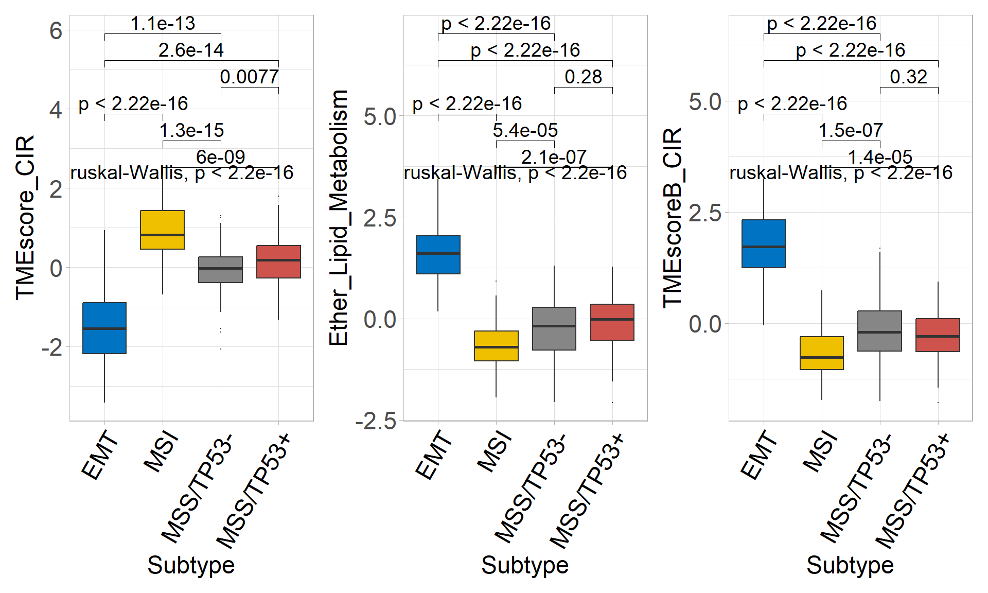
6.11 Reference
Cristescu, R., Lee, J., Nebozhyn, M. et al. Molecular analysis of gastric cancer identifies subtypes associated with distinct clinical outcomes. Nat Med 21, 449–456 (2015). https://doi.org/10.1038/nm.3850
Dongqiang Zeng, …, WJ Liao et al., Tumor Microenvironment Characterization in Gastric Cancer Identifies Prognostic and Immunotherapeutically Relevant Gene Signatures, Cancer Immunol Res (2019) 7 (5): 737–750. https://doi.org/10.1158/2326-6066.CIR-18-0436