Chapter 8 Tumor ecosystem analysis
8.2 Downloading data for example
Obtaining data set from GEO Gastric cancer: GSE62254 using GEOquery R package.
if (!requireNamespace("GEOquery", quietly = TRUE)) BiocManager::install("GEOquery")
library("GEOquery")
# NOTE: This process may take a few minutes which depends on the internet connection speed. Please wait for its completion.
eset_geo <- tryCatch(
  {
    getGEO(GEO = "GSE62254", getGPL = F, destdir = "./")
  },
  error = function(e) {
    message("Cannot download GSE62254 from GEO: ", e$message)
    message("Using eset_example1 from IOBR package instead...")
    NULL
  }
)

if (is.null(eset_geo)) {
  # Use eset_example1 as fallback - it has samples as rows and genes as columns
  eset <- t(eset_example1)
} else {
  eset <- eset_geo[[1]]
  eset <- exprs(eset)
}
eset[1:5, 1:5]
## GSM1523727 GSM1523728 GSM1523729 GSM1523744 GSM1523745
## 1007_s_at 3.2176645 3.0624323 3.0279131 2.921683 2.8456013
## 1053_at 2.4050109 2.4394879 2.2442708 2.345916 2.4328582
## 117_at 1.4933412 1.8067380 1.5959665 1.839822 1.8326058
## 121_at 2.1965561 2.2812181 2.1865556 2.258599 2.1874363
## 1255_g_at 0.8698382 0.9502466 0.8125414 1.012860 0.94419938.3 Gene Annotation: HGU133PLUS-2 (Affaymetrix)
# Gene annotation is only needed for GEO data (probe IDs)
# eset_example1 already has gene symbols, so skip annotation when using fallback
if (!is.null(eset_geo)) {
  # Conduct gene annotation using `anno_hug133plus2` file
  anno_hug133plus2 <- load_data("anno_hug133plus2")
  eset <- anno_eset(
    eset = eset,
    annotation = anno_hug133plus2,
    symbol = "symbol",
    probe = "probe_id",
    method = "mean"
  )
}
eset[1:5, 1:3]
## GSM1523727 GSM1523728 GSM1523729
## SH3KBP1 4.327974 4.316195 4.351425
## RPL41 4.246149 4.246808 4.257940
## EEF1A1 4.293762 4.291038 4.262199
## COX2 4.250288 4.283714 4.270508
## LOC101928826 4.219303 4.219670 4.2132528.4 Determine TME subtype of gastric cancer using TMEclassifier R package
if (!requireNamespace("TMEclassifier", quietly = TRUE)) remotes::install_github("LiaoWJLab/TMEclassifier", dependencies = TRUE)
# Specified version of xgboost
# install.packages("https://cran.r-project.org/src/contrib/Archive/xgboost/xgboost_1.5.2.1.tar.gz", repos = NULL)
library(TMEclassifier)
tme <- tme_classifier(eset = eset, scale = TRUE)
## Step-1: Expression data preprocessing...## Step-2: TME deconvolution...## Step-3: Predicting TME phenotypes...## >>>--- DONE!##
## IA IE IS
## 107 96 97## ID IE IS IA TMEcluster
## 1 GSM1523727 0.204623557 0.11212681 0.68324962 IA
## 2 GSM1523728 0.009599504 0.11179146 0.87860903 IA
## 3 GSM1523729 0.852615046 0.11369089 0.03369407 IE
## 4 GSM1523744 0.053842233 0.06994632 0.87621145 IA
## 5 GSM1523745 0.055973019 0.80839488 0.13563209 IS
## 6 GSM1523746 0.545343299 0.37437568 0.08028102 IE8.5 DEG analysis: method1
Differential analysis of selected immune-activated and immune-expelled gastric cancers
pdata <- tme[!tme$TMEcluster == "IS", ]
deg <- iobr_deg(
  eset = eset,
  annotation = NULL,
  pdata = pdata,
  group_id = "TMEcluster",
  pdata_id = "ID",
  array = TRUE,
  method = "limma",
  contrast = c("IA", "IE"),
  path = "result",
  padj_cutoff = 0.01,
  logfc_cutoff = 0.5
)
## ℹ Matching grouping information and expression matrix## ℹ Using limma for array differential analysis## ℹ Group 1 = IA## ℹ Group 2 = IE## ✔ DEG results written to: '/Users/wsx/Documents/GitHub/book/result/2-DEGs.csv'8.6 GSEA analysis based on differential express gene analysis results
Select the gene set list in IOBR’s signature collection.
## # A tibble: 6 × 11
##   symbol  log2FoldChange AveExpr     t   pvalue     padj     B sigORnot    label
##   <chr>            <dbl>   <dbl> <dbl>    <dbl>    <dbl> <dbl> <chr>       <chr>
## 1 TMEM100         -0.774    1.84 -13.9 2.47e-31 5.37e-27  60.4 Down_regul… Both
## 2 ABCA8           -0.933    1.90 -12.9 3.11e-28 3.38e-24  53.4 Down_regul… Both
## 3 HHIP            -0.613    1.73 -12.1 7.62e-26 4.46e-22  48.0 Down_regul… Both
## 4 LMNB2            0.287    2.25  12.1 9.28e-26 4.46e-22  47.8 NOT         Sign…
## 5 MCM6             0.211    3.02  12.1 1.02e-25 4.46e-22  47.7 NOT         Sign…
## 6 ADH1B           -0.907    1.86 -12.0 2.27e-25 7.04e-22  47.0 Down_regul… Both
## # ℹ 2 more variables: IA <dbl>, IE <dbl>
signature_collection <- load_data("signature_collection")
sig_list <- signature_collection[c(
"TMEscoreB_CIR", "TMEscoreA_CIR", "DNA_replication", "Base_excision_repair",
"Pan_F_TBRs", "TGFb.myCAF", "Ferroptosis", "TLS_Nature", "Glycolysis"
)]gsea <- sig_gsea(deg,
genesets = sig_list,
path = "result",
gene_symbol = "symbol",
logfc = "log2FoldChange",
org = "hsa",
show_plot = FALSE,
msigdb = TRUE,
category = "H",
subcategory = NULL,
palette_bar = "set2"
)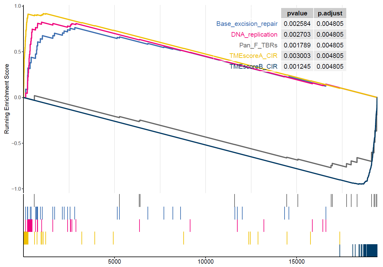
Figure 4.1: GSEA of TME gent sets
Hallmark gene signatures
gsea <- sig_gsea(deg,
  genesets          = NULL,
  path              = "GSEA",
  gene_symbol       = "symbol",
  logfc             = "log2FoldChange",
  org               = "hsa",
  show_plot         = FALSE,
  msigdb            = TRUE,
  category          = "H",
  subcategory       = NULL,
  palette_bar       = "aaas",
  show_bar          = 5,
  show_gsea         = 6
)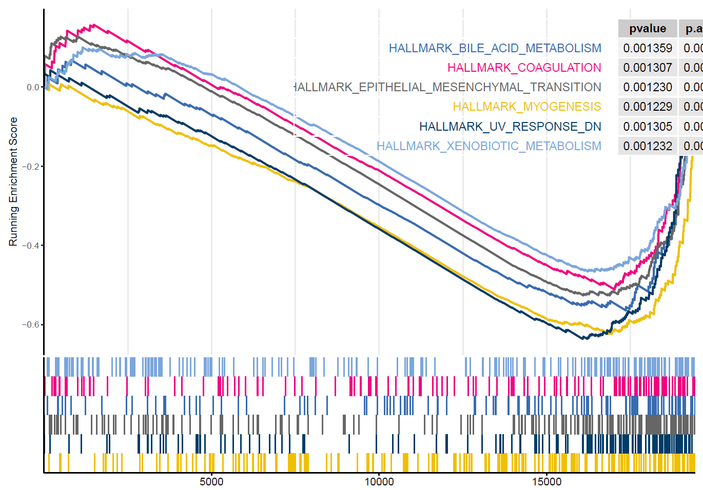
Figure 8.1: GSEA of Hallmark gent sets
8.7 DEG analysis: method2
Identifing TME subtype-related differential genes using alternative approach (ANOVA-based)
library(Seurat)
res <- find_markers_in_bulk(
  pdata = tme,
  eset = eset,
  group = "TMEcluster",
  nfeatures = 2000,
  top_n = 50,
  thresh.use = 0.15,
  only.pos = TRUE,
  min.pct = 0.10
)
top15 <- res$top_markers %>%
  dplyr::group_by(cluster) %>%
  dplyr::top_n(15, avg_log2FC)
top15$gene
## [1] "IDO1" "CXCL11" "SLCO1B3" "IFNG"
## [5] "AIM2" "GZMB" "VSNL1" "CXCL10"
## [9] "CXCL9" "GBP4" "KLRC2" "GNLY"
## [13] "GZMH" "KISS1R" "WARS" "C2orf40"
## [17] "OGN" "PGA4" "SCN7A" "C7"
## [21] "ADH1B" "GIF" "SCRG1" "LIPF"
## [25] "GHRL" "MAMDC2" "VIP" "ABCA8"
## [29] "ATP4A" "TMEM100" "REG1B" "MAGEA12"
## [33] "MAGEA4" "IL1A" "PI15" "IL11"
## [37] "MAGEA6" "MAGEA10-MAGEA5" "PPBP" "PROK2"
## [41] "MAGEA2B" "CLEC5A" "IL24" "CTAG1A"
## [45] "EREG"Heatmap visualisation using Seurat’s DoHeatmap
# 定义分型对应的颜色
cols <- c("#2692a4", "#fc0d3a", "#ffbe0b")
p1 <- DoHeatmap(res$sce, top15$gene, group.colors = cols) +
  scale_fill_gradientn(colours = rev(colorRampPalette(RColorBrewer::brewer.pal(11, "RdBu"))(256)))
Extracting variables from the expression matrix to merge with TME subtypes
input <- combine_pd_eset(eset = eset, pdata = tme, feas = top15$gene, scale = T)
p2 <- sig_box(input,
  variable = "TMEcluster", signature = "IFNG", jitter = TRUE,
  cols = cols, size_of_pvalue = 4
)
## Warning: The `size` argument of `element_line()` is deprecated as of ggplot2 3.4.0.
## ℹ Please use the `linewidth` argument instead.
## ℹ The deprecated feature was likely used in the IOBR package.
## Please report the issue at <https://github.com/IOBR/IOBR/issues>.
## This warning is displayed once per session.
## Call `lifecycle::last_lifecycle_warnings()` to see where this warning was
## generated.## # A tibble: 3 × 8
## .y. group1 group2 p p.adj p.format p.signif method
## <chr> <chr> <chr> <dbl> <dbl> <chr> <chr> <chr>
## 1 signature IA IE 4.09e-17 1.20e-16 < 2e-16 **** Wilcoxon
## 2 signature IA IS 1.44e-13 2.90e-13 1.4e-13 **** Wilcoxon
## 3 signature IE IS 8.35e- 2 8.4 e- 2 0.084 ns Wilcoxonp3 <- sig_box(input,
variable = "TMEcluster", signature = "IL1A",
jitter = TRUE, cols = cols, size_of_pvalue = 4
)## # A tibble: 3 × 8
## .y. group1 group2 p p.adj p.format p.signif method
## <chr> <chr> <chr> <dbl> <dbl> <chr> <chr> <chr>
## 1 signature IA IE 1.46e-10 2.90e-10 1.5e-10 **** Wilcoxon
## 2 signature IA IS 8.22e- 7 8.2 e- 7 8.2e-07 **** Wilcoxon
## 3 signature IE IS 4.90e-20 1.5 e-19 < 2e-16 **** Wilcoxonif (!requireNamespace("patchwork", quietly = TRUE)) install.packages("patchwork")
library(patchwork)
p <- (p1 | p2 / p3) + plot_layout(widths = c(2.3, 1))
p + plot_annotation(tag_levels = "A")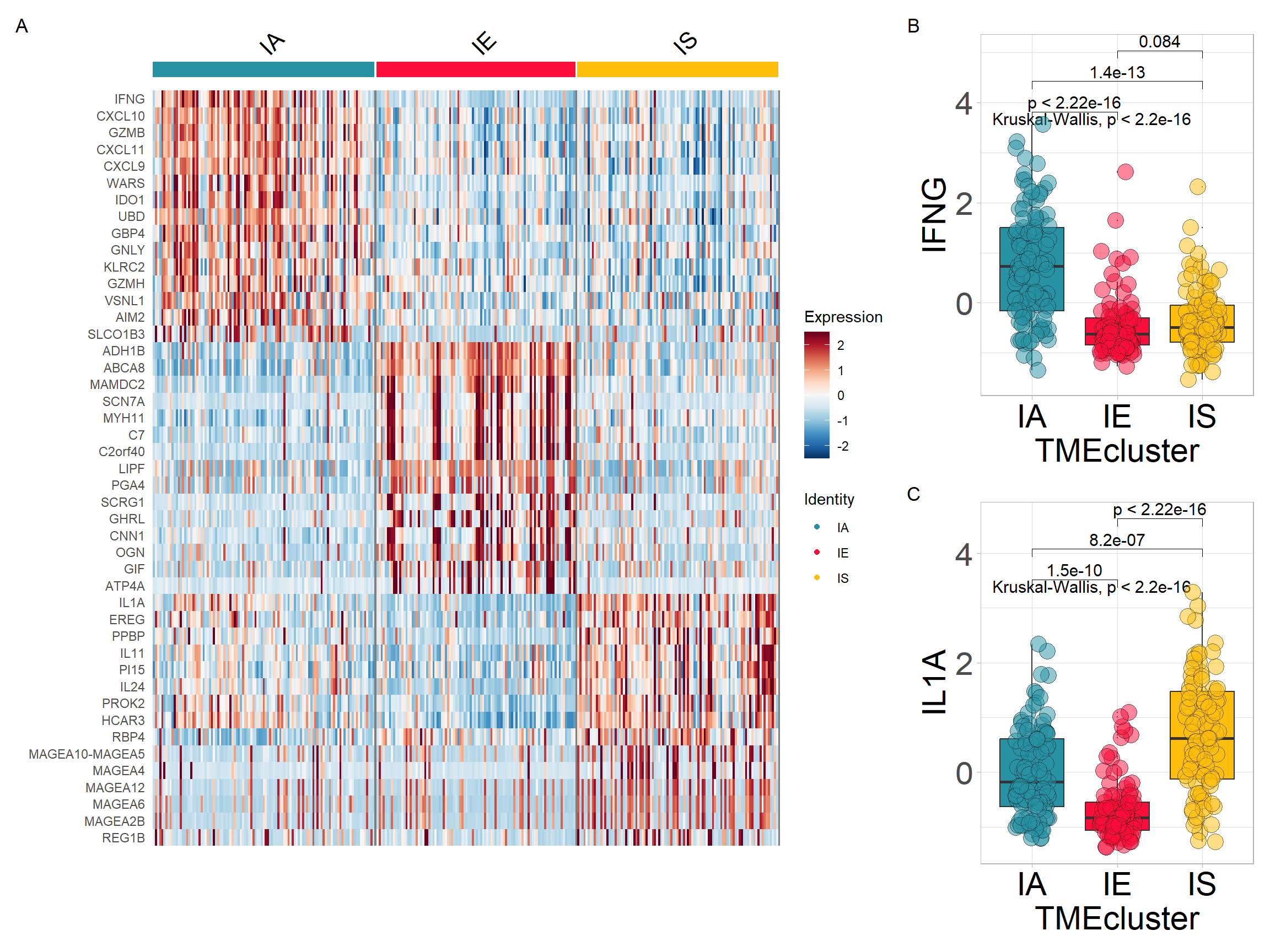
8.8 Identifying signatures associated with TME clusters
Calculate TME associated signatures-(through PCA method).
sig_tme <- calculate_sig_score(
  pdata = NULL,
  eset = eset,
  signature = signature_collection,
  method = "pca",
  mini_gene_count = 2
)
sig_tme <- t(column_to_rownames(sig_tme, var = "ID"))
sig_tme[1:5, 1:3]
## GSM1523727 GSM1523728 GSM1523729
## CD_8_T_effector -2.5513794 0.7789141 -2.1770675
## DDR -0.8747614 0.7425162 -1.3272054
## APM 1.1098368 2.1988688 -0.9516419
## Immune_Checkpoint -2.3701787 0.9455120 -1.4844104
## CellCycle_Reg 0.1063358 0.7583302 -0.3649795Finding signatures or cell types associated with TMEcluster
res <- find_markers_in_bulk(pdata = tme, eset = sig_tme, group = "TMEcluster", nfeatures = 1000, top_n = 20, min.pct = 0.10)

top15 <- res$top_markers %>%
  dplyr::group_by(cluster) %>%
  dplyr::top_n(15, avg_log2FC)

p1 <- DoHeatmap(res$sce, top15$gene, group.colors = cols) +
scale_fill_gradientn(colours = rev(colorRampPalette(RColorBrewer::brewer.pal(11, "RdBu"))(256)))top15$gene <- gsub(top15$gene, pattern = "-", replacement = "\\_")
input <- combine_pd_eset(eset = sig_tme, pdata = tme, feas = top15$gene, scale = T)
p2 <- sig_box(input,
variable = "TMEcluster", signature = "CD_8_T_effector", jitter = TRUE,
cols = cols, size_of_pvalue = 4, size_of_font = 6
)## # A tibble: 3 × 8
## .y. group1 group2 p p.adj p.format p.signif method
## <chr> <chr> <chr> <dbl> <dbl> <chr> <chr> <chr>
## 1 signature IA IE 3.53e-10 7.10e-10 3.5e-10 **** Wilcoxon
## 2 signature IA IS 8.49e-13 2.5 e-12 8.5e-13 **** Wilcoxon
## 3 signature IE IS 1.41e- 1 1.4 e- 1 0.14 ns Wilcoxonp3 <- sig_box(input,
variable = "TMEcluster", signature = "Neutrophils_Bindea_et_al",
jitter = TRUE, cols = cols, size_of_pvalue = 4, size_of_font = 6
)## # A tibble: 3 × 8
## .y. group1 group2 p p.adj p.format p.signif method
## <chr> <chr> <chr> <dbl> <dbl> <chr> <chr> <chr>
## 1 signature IA IE 0.00639 0.013 0.0064 ** Wilcoxon
## 2 signature IA IS 0.0584 0.058 0.0584 ns Wilcoxon
## 3 signature IE IS 0.0000929 0.00028 9.3e-05 **** Wilcoxon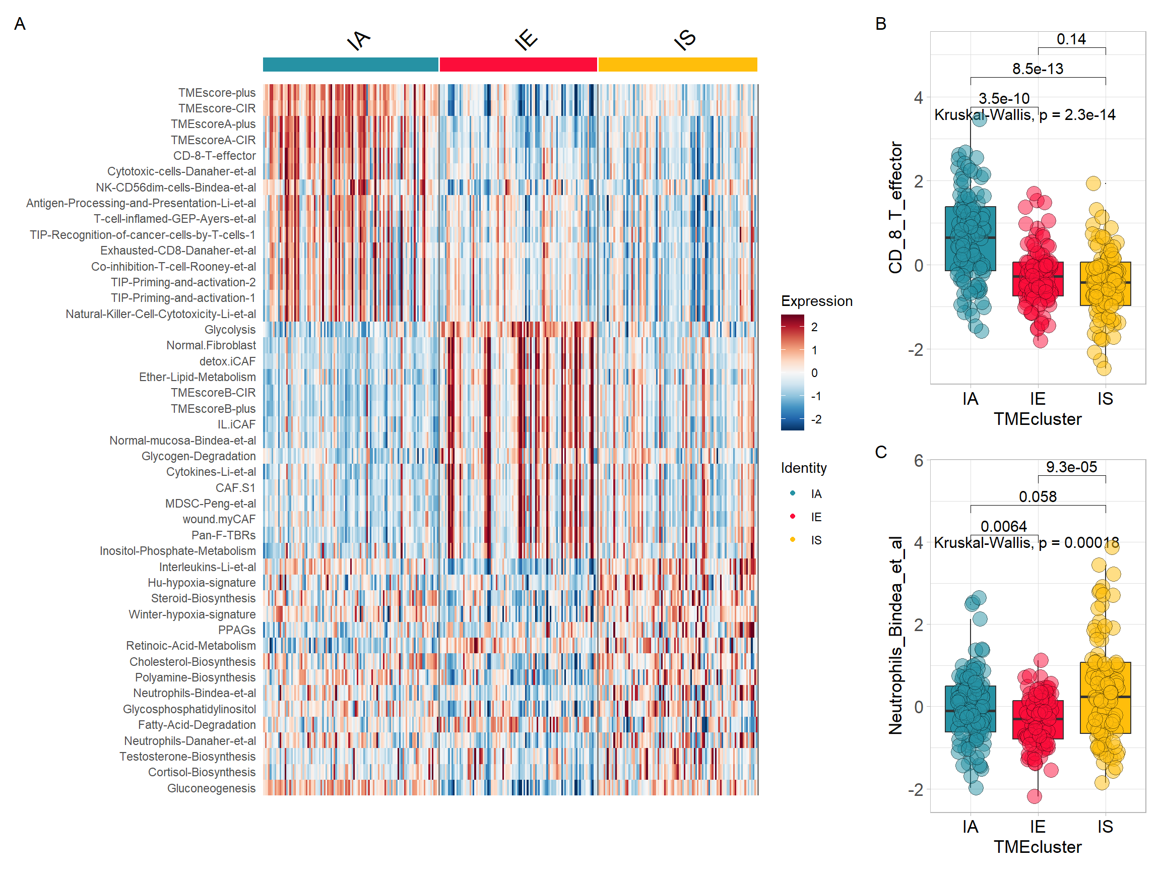
## Loading required package: ggpubr## ℹ Loading cached data: "pdata_acrg"input <- merge(pdata_acrg, input, by = "ID")
p1 <- surv_group(
input_pdata = input,
target_group = "TMEcluster",
ID = "ID",
reference_group = "High",
project = "ACRG",
cols = cols,
time = "OS_time",
status = "OS_status",
time_type = "month",
save_path = "result"
)## ℹ Follow-up time ranges from 1 to 105.7 months## IA IE IS
## 107 96 97## ℹ Maximum follow-up time is 105.7 months; divided into 6 sections## Registered S3 methods overwritten by 'ggpp':
## method from
## heightDetails.titleGrob ggplot2
## widthDetails.titleGrob ggplot2## Ignoring unknown labels:
## • colour : "Strata"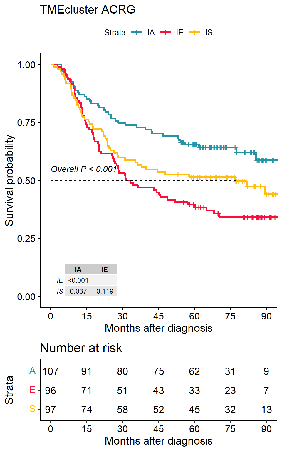
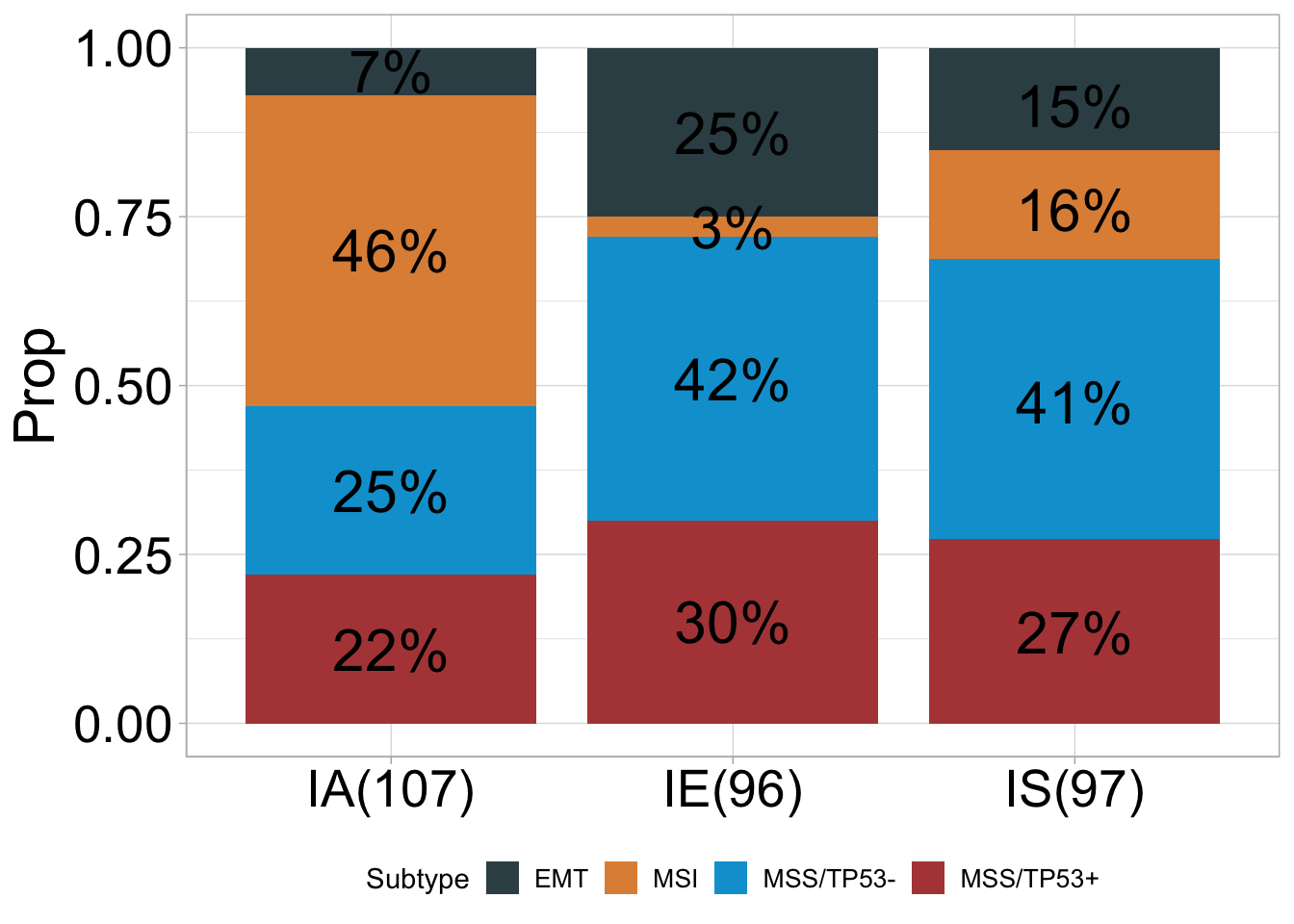
## # A tibble: 12 × 5
## # Groups: TMEcluster [3]
## TMEcluster Subtype Freq Prop count
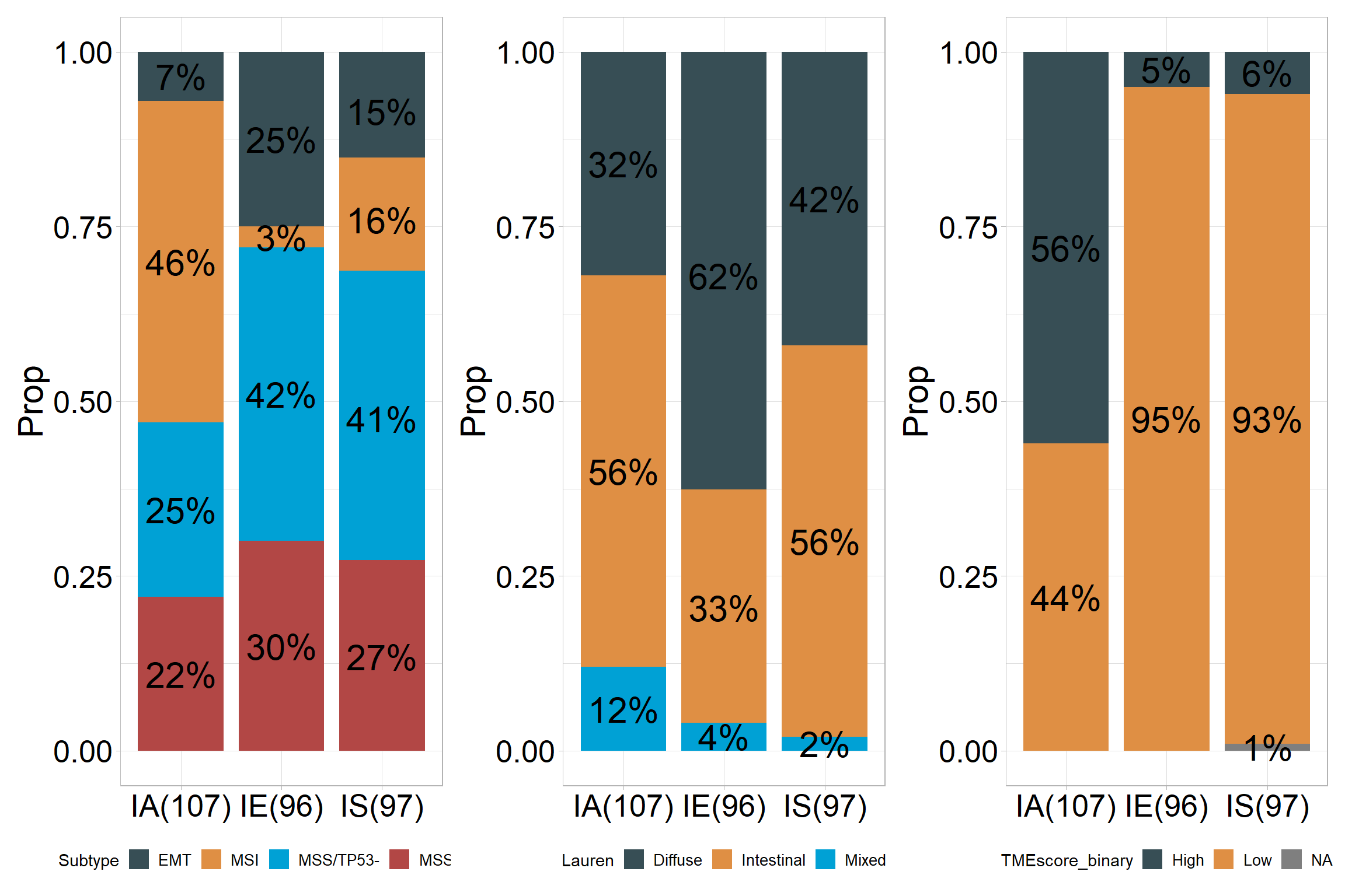
## <chr> <fct> <dbl> <dbl> <dbl>
## 1 IA EMT 7 0.07 107
## 2 IA MSI 49 0.46 107
## 3 IA MSS/TP53- 27 0.25 107
## 4 IA MSS/TP53+ 24 0.22 107
## 5 IE EMT 24 0.25 96
## 6 IE MSI 3 0.03 96
## 7 IE MSS/TP53- 40 0.42 96
## 8 IE MSS/TP53+ 29 0.3 96
## 9 IS EMT 15 0.15 97
## 10 IS MSI 16 0.16 97
## 11 IS MSS/TP53- 40 0.41 97
## 12 IS MSS/TP53+ 26 0.27 97## ℹ Available categories: box, continue2, continue, random, heatmap, heatmap3, tidyheatmap## ℹ Box palettes: nrc, jama, aaas, jco, paired1, paired2, paired3, paired4, accent, set2## [1] "'#374E55FF', '#DF8F44FF', '#00A1D5FF', '#B24745FF', '#79AF97FF', '#6A6599FF', '#80796BFF'"
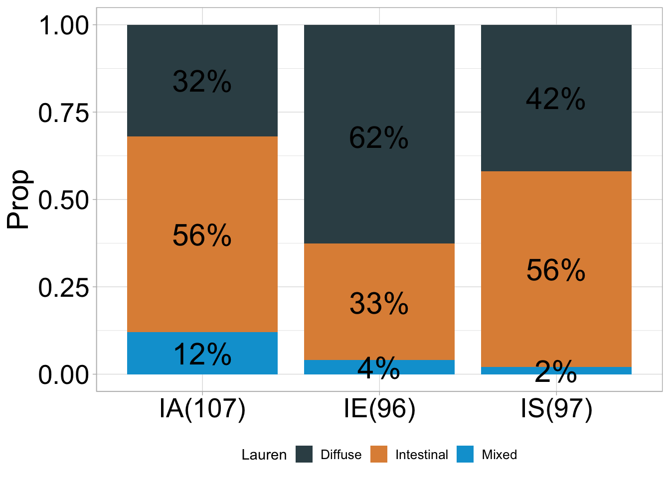
## # A tibble: 9 × 5
## # Groups:   TMEcluster [3]
##   TMEcluster Lauren      Freq  Prop count
##   <chr>      <fct>      <dbl> <dbl> <dbl>
## 1 IA         Diffuse       34  0.32   107
## 2 IA         Intestinal    60  0.56   107
## 3 IA         Mixed         13  0.12   107
## 4 IE         Diffuse       60  0.62    96
## 5 IE         Intestinal    32  0.33    96
## 6 IE         Mixed          4  0.04    96
## 7 IS         Diffuse       41  0.42    97
## 8 IS         Intestinal    54  0.56    97
## 9 IS         Mixed          2  0.02    97
## ℹ Available categories: box, continue2, continue, random, heatmap, heatmap3, tidyheatmap
## ℹ Box palettes: nrc, jama, aaas, jco, paired1, paired2, paired3, paired4, accent, set2## [1] "'#374E55FF', '#DF8F44FF', '#00A1D5FF', '#B24745FF', '#79AF97FF', '#6A6599FF', '#80796BFF'"
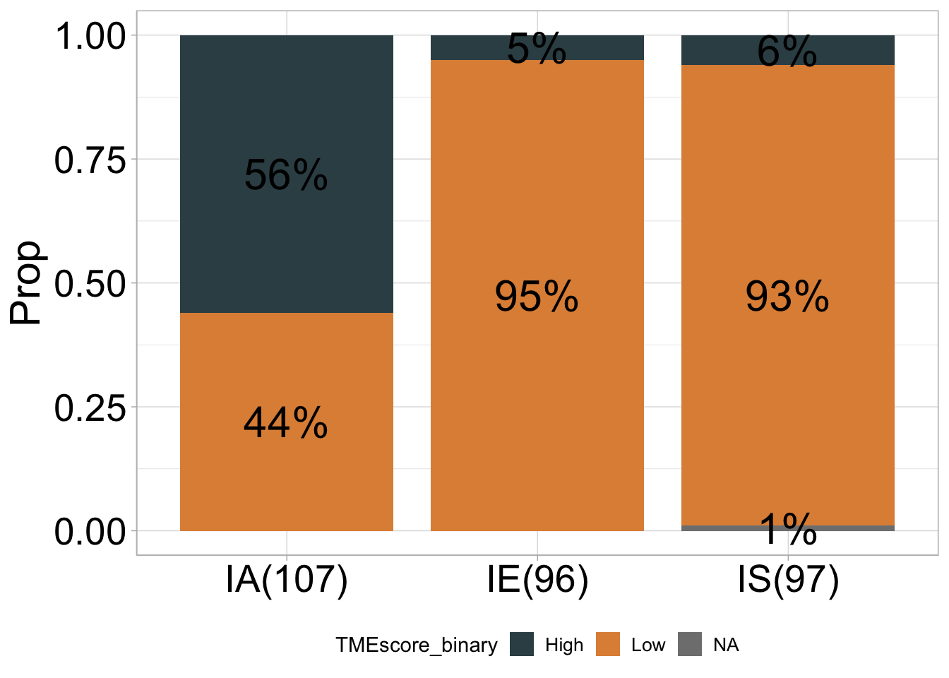
## # A tibble: 7 × 5
## # Groups:   TMEcluster [3]
##   TMEcluster TMEscore_binary  Freq  Prop count
##   <chr>      <fct>           <dbl> <dbl> <dbl>
## 1 IA         High               60  0.56   107
## 2 IA         Low                47  0.44   107
## 3 IE         High                5  0.05    96
## 4 IE         Low                91  0.95    96
## 5 IS         High                6  0.06    97
## 6 IS         Low                90  0.93    97
## 7 IS         <NA>                1  0.01    97
## ℹ Available categories: box, continue2, continue, random, heatmap, heatmap3, tidyheatmap
## ℹ Box palettes: nrc, jama, aaas, jco, paired1, paired2, paired3, paired4, accent, set2## [1] "'#374E55FF', '#DF8F44FF', '#00A1D5FF', '#B24745FF', '#79AF97FF', '#6A6599FF', '#80796BFF'"
8.9 References
Cristescu, R., Lee, J., Nebozhyn, M. et al. Molecular analysis of gastric cancer identifies subtypes associated with distinct clinical outcomes. Nat Med 21, 449–456 (2015). https://doi.org/10.1038/nm.3850
CIBERSORT; Newman, A. M., Liu, C. L., Green, M. R., Gentles, A. J., Feng, W., Xu, Y., … Alizadeh, A. A. (2015). Robust enumeration of cell subsets from tissue expression profiles. Nature Methods, 12(5), 453–457. https://doi.org/10.1038/nmeth.3337;
Seurat: Hao and Hao et al. Integrated analysis of multimodal single-cell data. Cell (2021)
Zeng D, Yu Y, Qiu W, Mao Q, …, Zhang K, Liao W; Tumor microenvironment immunotyping heterogeneity reveals distinct molecular mechanisms to clinical immunotherapy applications in gastric cancer. (2024) Under Review.