Chapter 7 TME Interaction analysis
7.2 Downloading data for example
Obtaining data set from GEO Gastric cancer: GSE62254 using GEOquery R package.
if (!requireNamespace("GEOquery", quietly = TRUE)) BiocManager::install("GEOquery")
library("GEOquery")
# NOTE: This process may take a few minutes which depends on the internet connection speed. Please wait for its completion.
eset_geo <- getGEO(GEO = "GSE62254", getGPL = F, destdir = "./")
eset <- eset_geo[[1]]
eset <- exprs(eset)
eset[1:5, 1:5]
## GSM1523727 GSM1523728 GSM1523729 GSM1523744 GSM1523745
## 1007_s_at 3.2176645 3.0624323 3.0279131 2.921683 2.8456013
## 1053_at 2.4050109 2.4394879 2.2442708 2.345916 2.4328582
## 117_at 1.4933412 1.8067380 1.5959665 1.839822 1.8326058
## 121_at 2.1965561 2.2812181 2.1865556 2.258599 2.1874363
## 1255_g_at 0.8698382 0.9502466 0.8125414 1.012860 0.94419937.3 Gene Annotation: HGU133PLUS-2 (Affaymetrix)
# Conduct gene annotation using `anno_hug133plus2` file; If identical gene symbols exists, these genes would be ordered by the mean expression levels. The gene symbol with highest mean expression level is selected and remove others.
anno_hug133plus2 <- load_data("anno_hug133plus2")
eset <- anno_eset(
  eset = eset,
  annotation = anno_hug133plus2,
  symbol = "symbol",
  probe = "probe_id",
  method = "mean"
)
eset[1:5, 1:3]
## GSM1523727 GSM1523728 GSM1523729
## SH3KBP1 4.327974 4.316195 4.351425
## RPL41 4.246149 4.246808 4.257940
## EEF1A1 4.293762 4.291038 4.262199
## COX2 4.250288 4.283714 4.270508
## LOC101928826 4.219303 4.219670 4.2132527.4 TME deconvolution using CIBERSORT algorithm
cell <- deconvo_tme(eset = eset, method = "cibersort", arrays = TRUE, perm = 500, absolute.mode = TRUE)
head(cell)
## # A tibble: 6 × 27
## ID B_cells_naive_CIBERS…¹ B_cells_memory_CIBER…² Plasma_cells_CIBERSORT
## <chr> <dbl> <dbl> <dbl>
## 1 GSM15237… 0.00610 0.0136 0.149
## 2 GSM15237… 0 0.0340 0.0764
## 3 GSM15237… 0.00335 0.0183 0.0939
## 4 GSM15237… 0 0.0594 0.0773
## 5 GSM15237… 0 0.00731 0.109
## 6 GSM15237… 0.0122 0.0113 0.138
## # ℹ abbreviated names: ¹B_cells_naive_CIBERSORT, ²B_cells_memory_CIBERSORT
## # ℹ 23 more variables: T_cells_CD8_CIBERSORT <dbl>,
## # T_cells_CD4_naive_CIBERSORT <dbl>,
## # T_cells_CD4_memory_resting_CIBERSORT <dbl>,
## # T_cells_CD4_memory_activated_CIBERSORT <dbl>,
## # T_cells_follicular_helper_CIBERSORT <dbl>,
## # `T_cells_regulatory_(Tregs)_CIBERSORT` <dbl>, …7.5 Identifying TME patterns
Identification of optimal clustering based on cellular infiltration patterns in the microenvironment.
tme <- tme_cluster(input = cell, features = colnames(cell)[2:23], id = "ID", scale = TRUE, method = "kmeans", max.nc = 5)## 1 2 3
## 85 96 119Use of heatmaps to reflect cellular differences between TME subtypes.
colnames(tme) <- gsub(colnames(tme), pattern = "_CIBERSORT", replacement = "")
res <- sig_heatmap(input = tme, features = colnames(tme)[3:ncol(tme)], group = "cluster", path = "result", palette = 6)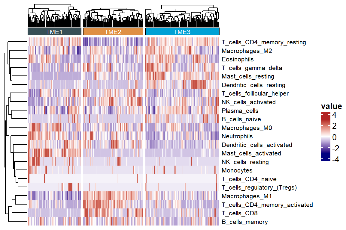
7.6 Cell abundance of each cluster
cols <- c("#2692a4", "#fc0d3a", "#ffbe0b")
p1 <- sig_box(tme,
  variable = "cluster", signature = "Macrophages_M1", jitter = TRUE,
  cols = cols, show_pairwise_p = TRUE, size_of_pvalue = 4
)
## # A tibble: 3 × 8
## .y. group1 group2 p p.adj p.format p.signif method
## <chr> <chr> <chr> <dbl> <dbl> <chr> <chr> <chr>
## 1 signature TME3 TME2 2.25e-17 4.50e-17 < 2e-16 **** Wilcoxon
## 2 signature TME3 TME1 3.48e- 6 3.5 e- 6 3.5e-06 **** Wilcoxon
## 3 signature TME2 TME1 6.50e-24 2 e-23 < 2e-16 **** Wilcoxonp2 <- sig_box(tme,
variable = "cluster", signature = "Mast_cells_activated",
jitter = TRUE, cols = cols, show_pairwise_p = TRUE, size_of_pvalue = 4
)## # A tibble: 3 × 8
## .y. group1 group2 p p.adj p.format p.signif method
## <chr> <chr> <chr> <dbl> <dbl> <chr> <chr> <chr>
## 1 signature TME3 TME2 1.91e- 1 1.9 e- 1 0.19 ns Wilcoxon
## 2 signature TME3 TME1 6.89e-33 2.10e-32 <2e-16 **** Wilcoxon
## 3 signature TME2 TME1 1.16e-25 2.3 e-25 <2e-16 **** Wilcoxonp3 <- sig_box(tme,
variable = "cluster", signature = "Macrophages_M2",
jitter = TRUE, cols = cols, show_pairwise_p = TRUE, size_of_pvalue = 4
)## # A tibble: 3 × 8
## .y. group1 group2 p p.adj p.format p.signif method
## <chr> <chr> <chr> <dbl> <dbl> <chr> <chr> <chr>
## 1 signature TME3 TME2 0.0997 0.1 0.09972 ns Wilcoxon
## 2 signature TME3 TME1 0.000518 0.0016 0.00052 *** Wilcoxon
## 3 signature TME2 TME1 0.0510 0.1 0.05101 ns Wilcoxon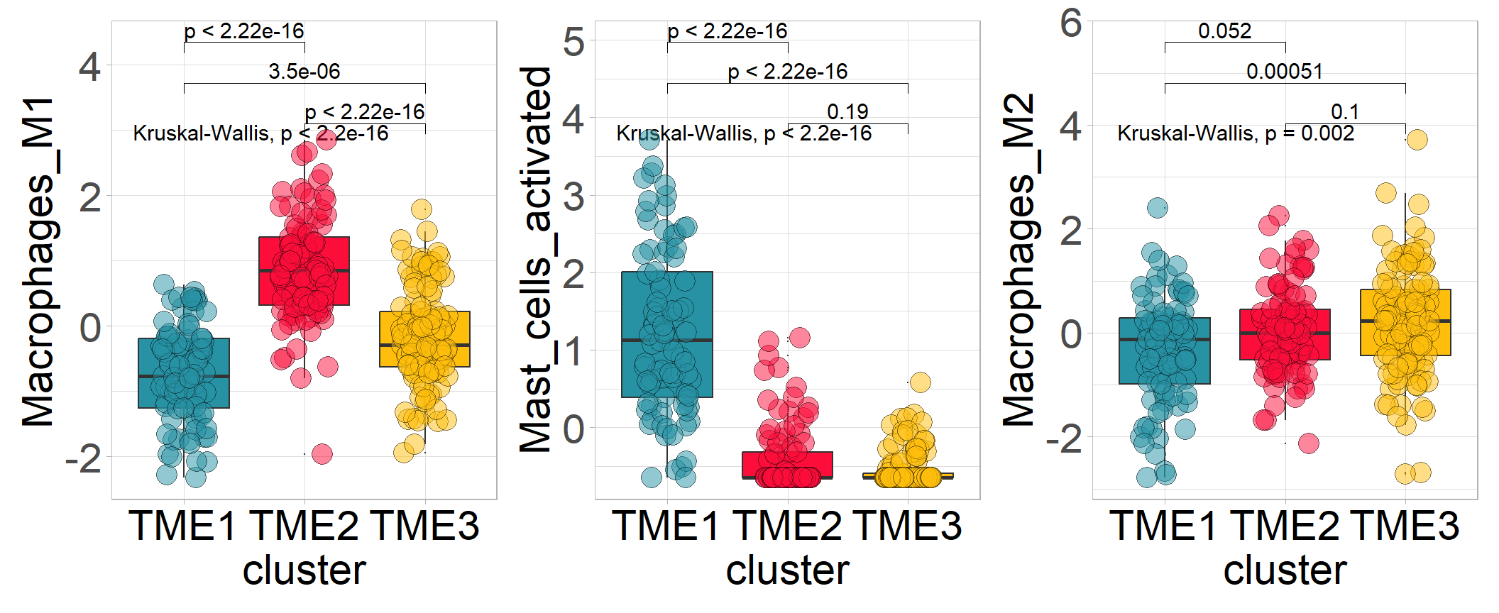
7.7 DEG analysis between TME subtypes
Identifying TME subtypes related differential genes using find_markers_in_bulk.
We have developed a reliable classifier for the tumour microenvironment in gastric cancer using the same analysis pipelineTMEclassifier. The classifier was constructed by identifying the most robust gastric cancer TME classification through parsing the tumour microenvironment using the tme_cluster method. Next, genes specifically expressed by each microenvironmental subtype are obtained using the find_markers_in_bulk method. Finally, a machine learning approach was used to construct the classifier model.
library(Seurat)
res <- find_markers_in_bulk(
  pdata = tme,
  eset = eset,
  group = "cluster",
  nfeatures = 2000,
  top_n = 50,
  thresh.use = 0.15,
  only.pos = TRUE,
  min.pct = 0.10
)
top15 <- res$top_markers %>%
  dplyr::group_by(cluster) %>%
  dplyr::top_n(15, avg_log2FC)
top15$gene
## [1] "C2orf40" "LIPF" "OGN" "ADH1B" "PGA4" "SCN7A"
## [7] "C7" "MAMDC2" "ABCA8" "GIF" "SCRG1" "C6orf58"
## [13] "VIP" "TMEM100" "GHRL" "IDO1" "CXCL11" "SLCO1B3"
## [19] "AIM2" "IFNG" "GZMB" "CXCL10" "GBP4" "KRT13"
## [25] "CXCL9" "GNLY" "S100A2" "COL11A1" "SERPINB2" "KISS1R"
## [31] "IL1A" "REG1B" "PROK2" "PI15" "IL11" "PPBP"
## [37] "CLEC5A" "MAGEA6" "MAGEA12" "IGFBP1" "TREM1" "HCAR3"
## [43] "IL24" "MAGEA2B" "CXCL6"Heatmap visualisation using Seurat’s DoHeatmap
# Defining cluster colors
cols <- c("#2692a4", "#fc0d3a", "#ffbe0b")
p1 <- DoHeatmap(res$sce, top15$gene, group.colors = cols) +
  scale_fill_gradientn(colours = rev(colorRampPalette(RColorBrewer::brewer.pal(11, "RdBu"))(256)))
Extracting variables from the expression matrix to merge with TME subtype
input <- combine_pd_eset(eset = eset, pdata = tme, feas = top15$gene, scale = T)
p2 <- sig_box(input,
  variable = "cluster", signature = "IFNG", jitter = TRUE,
  cols = cols, show_pairwise_p = TRUE, size_of_pvalue = 4
)
## # A tibble: 3 × 8
## .y. group1 group2 p p.adj p.format p.signif method
## <chr> <chr> <chr> <dbl> <dbl> <chr> <chr> <chr>
## 1 signature TME3 TME2 1.11e-16 3.30e-16 < 2e-16 **** Wilcoxon
## 2 signature TME3 TME1 6.70e- 1 6.7 e- 1 0.67 ns Wilcoxon
## 3 signature TME2 TME1 5.60e-14 1.10e-13 5.6e-14 **** Wilcoxonp3 <- sig_box(input,
variable = "cluster", signature = "IL1A",
jitter = TRUE, cols = cols, show_pairwise_p = TRUE, size_of_pvalue = 4
)## # A tibble: 3 × 8
## .y. group1 group2 p p.adj p.format p.signif method
## <chr> <chr> <chr> <dbl> <dbl> <chr> <chr> <chr>
## 1 signature TME3 TME2 5.94e- 9 1.20e- 8 5.9e-09 **** Wilcoxon
## 2 signature TME3 TME1 7.96e-18 2.40e-17 < 2e-16 **** Wilcoxon
## 3 signature TME2 TME1 2.60e- 5 2.6 e- 5 2.6e-05 **** WilcoxonCombining the results obtained above
# if (!requireNamespace("patchwork", quietly = TRUE))   install.packages("patchwork")
library(patchwork)
p <- (p1 | p2 / p3) + plot_layout(widths = c(2.3, 1))
p + plot_annotation(tag_levels = "A")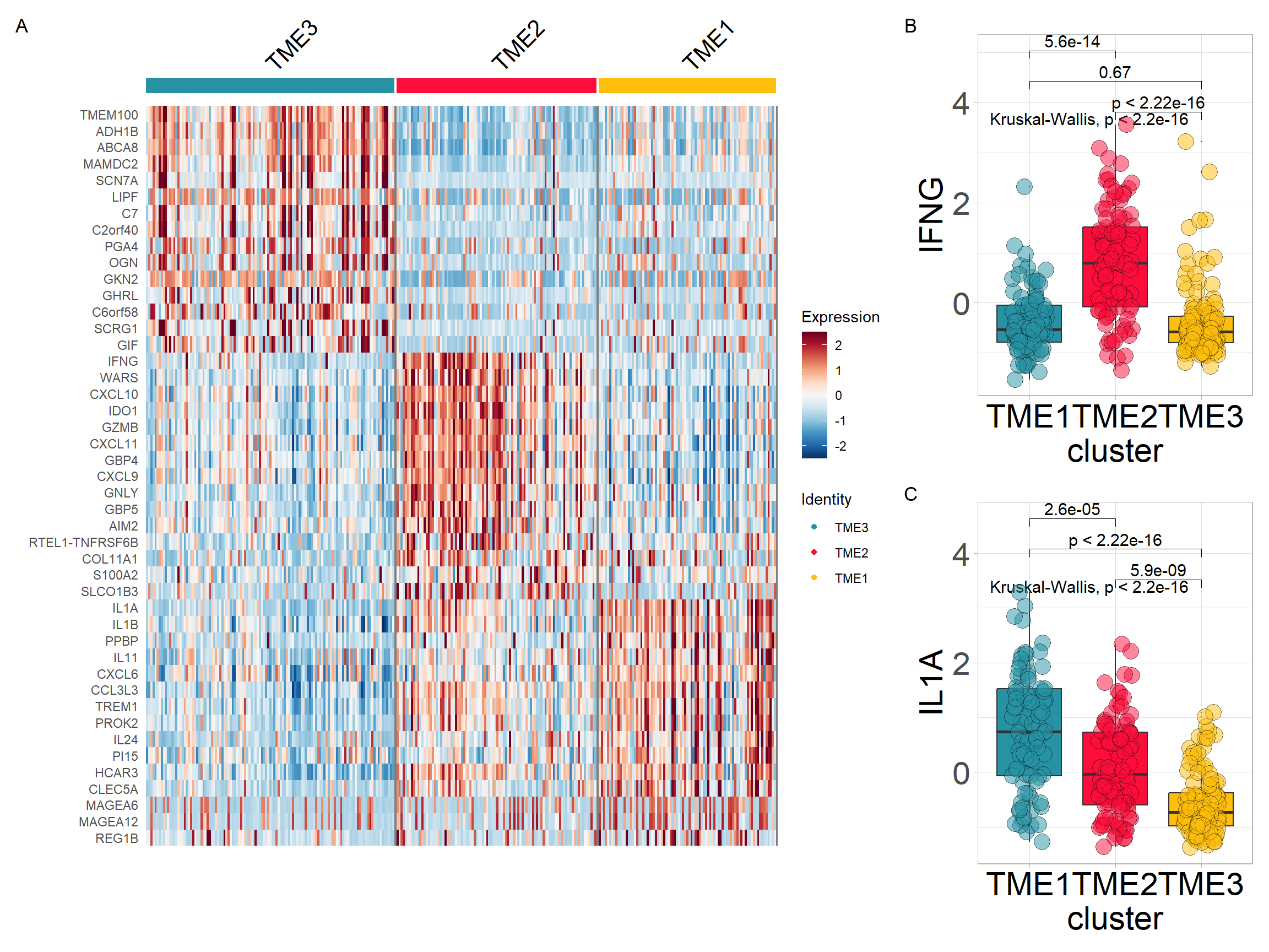
7.8 Identifying LR associated with TME clusters
The LR_cal method originates from the study:
Lapuente-Santana, Ó., van Genderen, M., Hilbers, P., Finotello, F., & Eduati, F. (2021). “Interpretable systems biomarkers predict response to immune-checkpoint inhibitors.” Patterns (New York, N.Y.), 2(8), 100293. DOI: 10.1016/j.patter.2021.100293.
The method calculates interaction weights for 813 ligand-receptor (LR) pairs. For this function to run successfully, you need to install the easier package following the tutorial available at easier GitHub repository.
lr <- column_to_rownames(lr_data, var = "ID") %>%
  t() %>%
  as.data.frame()
res <- find_markers_in_bulk(
  pdata = tme,
  eset = lr,
  group = "cluster",
  nfeatures = 2000,
  top_n = 50,
  thresh.use = 0.15,
  only.pos = TRUE,
  min.pct = 0.10
)
top15 <- res$top_markers %>%
  dplyr::group_by(cluster) %>%
  dplyr::top_n(15, avg_log2FC)
top15$gene
## [1] "ANGPTL1-TEK" "FN1-ITGA8" "COL4A5-CD93"
## [4] "GNAI2-P2RY12" "NCAM1-GFRA1" "FGF7-FGFR1-NRP1"
## [7] "LTF-LRP11" "SFRP1-FZD6" "MYOC-FZD4"
## [10] "EFNB2-EPHA3" "ADAM10-EFNA1-EPHA3" "MYOC-FZD1"
## [13] "TSLP-IL7R" "NCAM1-FGFR1" "F13A1-ITGA9"
## [16] "IFNG-IFNGR1-IFNGR2" "GZMB-IGF2R" "HLA-B-HLA-E-KLRD1"
## [19] "CXCL10-SDC4" "FASLG-FAS" "CCL7-CCR1"
## [22] "CCL7-CCR5" "CCL8-CCR5" "CCL5-SDC4"
## [25] "CCL7-ACKR4" "CCL8-CCR1" "CCL7-CCR2"
## [28] "CCL7-CXCR3" "TNFSF9-TNFRSF9" "IL15-IL2RA"
## [31] "IL1A-IL1R1" "IL1A-IL1R2" "PPBP-CXCR2"
## [34] "IL1A-IL1RAP" "FN1-TNFRSF11B" "THBS1-TNFRSF11B"
## [37] "TNFSF10-TNFRSF11B" "OSM-IL6ST" "PPBP-CXCR1"
## [40] "VWF-TNFRSF11B" "EREG-EGFR" "OSM-OSMR"
## [43] "TNFSF13-TNFRSF11B" "IL6-IL6ST" "ANXA1-APP-FPR2"Heatmap visualisation using Seurat’s DoHeatmap
# cols <- c('#2692a4','#fc0d3a','#ffbe0b')
p1 <- DoHeatmap(res$sce, top15$gene, group.colors = cols) +
  scale_fill_gradientn(colours = rev(colorRampPalette(RColorBrewer::brewer.pal(11, "RdBu"))(256)))
## Scale for fill is already present.
## Adding another scale for fill, which will replace the existing scale.Extracting variables from the expression matrix to merge with TME subtype.
top15$gene <- gsub(top15$gene, pattern = "-", replacement = "\\_")
input <- combine_pd_eset(eset = lr, pdata = tme, feas = top15$gene, scale = T)

p2 <- sig_box(input,
  variable = "cluster", signature = top15$gene[1], jitter = TRUE,
  cols = cols, show_pairwise_p = TRUE, size_of_pvalue = 4
)
## # A tibble: 3 × 8
## .y. group1 group2 p p.adj p.format p.signif method
## <chr> <chr> <chr> <dbl> <dbl> <chr> <chr> <chr>
## 1 signature TME3 TME2 0.000000823 0.0000025 8.2e-07 **** Wilcoxon
## 2 signature TME3 TME1 0.0000336 0.000067 3.4e-05 **** Wilcoxon
## 3 signature TME2 TME1 0.649 0.65 0.65 ns Wilcoxonp3 <- sig_box(input,
variable = "cluster", signature = top15$gene[5],
jitter = TRUE, cols = cols, show_pairwise_p = TRUE, size_of_pvalue = 4
)## # A tibble: 3 × 8
## .y. group1 group2 p p.adj p.format p.signif method
## <chr> <chr> <chr> <dbl> <dbl> <chr> <chr> <chr>
## 1 signature TME3 TME2 5.86e-16 1.80e-15 5.9e-16 **** Wilcoxon
## 2 signature TME3 TME1 1.31e-10 2.6 e-10 1.3e-10 **** Wilcoxon
## 3 signature TME2 TME1 1.14e- 1 1.1 e- 1 0.11 ns WilcoxonCombining the results obtained above.
# if (!requireNamespace("patchwork", quietly = TRUE))   install.packages("patchwork")
library(patchwork)
p <- (p1 | p2 / p3) + plot_layout(widths = c(2.3, 1))
p + plot_annotation(tag_levels = "A")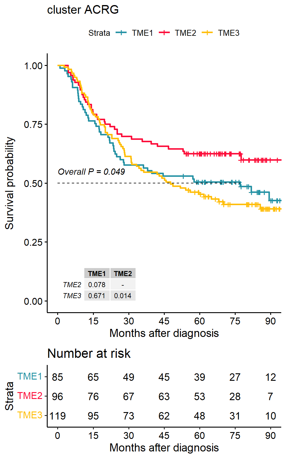
7.9 Identifying signatures associated with TME clusters
Calculate TME associated signatures-(through PCA method).
signature_collection <- load_data("signature_collection")
sig_tme <- calculate_sig_score(
  pdata = NULL,
  eset = eset,
  signature = signature_collection,
  method = "pca",
  mini_gene_count = 2
)
sig_tme <- t(column_to_rownames(sig_tme, var = "ID"))
sig_tme[1:5, 1:3]
## GSM1523727 GSM1523728 GSM1523729
## CD_8_T_effector -2.5513794 0.7789141 -2.1770675
## DDR -0.8747614 0.7425162 -1.3272054
## APM 1.1098368 2.1988688 -0.9516419
## Immune_Checkpoint -2.3701787 0.9455120 -1.4844104
## CellCycle_Reg 0.1063358 0.7583302 -0.3649795Finding characteristic variables associated with TME clusters.
res <- find_markers_in_bulk(pdata = tme, eset = sig_tme, group = "cluster", nfeatures = 1000, top_n = 20, min.pct = 0.10)

top15 <- res$top_markers %>%
  dplyr::group_by(cluster) %>%
  dplyr::top_n(15, avg_log2FC)

p1 <- DoHeatmap(res$sce, top15$gene, group.colors = cols) +
  scale_fill_gradientn(colours = rev(colorRampPalette(RColorBrewer::brewer.pal(11, "RdBu"))(256)))
Visualizing results and selecting feature variables
top15$gene <- gsub(top15$gene, pattern = "-", replacement = "\\_")
input <- combine_pd_eset(eset = sig_tme, pdata = tme, feas = top15$gene, scale = T)

p2 <- sig_box(input,
  variable = "cluster", signature = "CD_8_T_effector", jitter = TRUE,
  cols = cols, show_pairwise_p = TRUE, size_of_pvalue = 4, size_of_font = 6
)
## # A tibble: 3 × 8
## .y. group1 group2 p p.adj p.format p.signif method
## <chr> <chr> <chr> <dbl> <dbl> <chr> <chr> <chr>
## 1 signature TME3 TME2 3.18e-12 6.40e-12 3.2e-12 **** Wilcoxon
## 2 signature TME3 TME1 1.01e- 1 1 e- 1 0.1 ns Wilcoxon
## 3 signature TME2 TME1 4.53e-13 1.4 e-12 4.5e-13 **** Wilcoxonp3 <- sig_box(input,
variable = "cluster", signature = "Neutrophils_Bindea_et_al",
jitter = TRUE, cols = cols, show_pairwise_p = TRUE, size_of_pvalue = 4, size_of_font = 6
)## # A tibble: 3 × 8
## .y. group1 group2 p p.adj p.format p.signif method
## <chr> <chr> <chr> <dbl> <dbl> <chr> <chr> <chr>
## 1 signature TME3 TME2 0.0000416 0.000097 4.2e-05 **** Wilcoxon
## 2 signature TME3 TME1 0.0000323 0.000097 3.2e-05 **** Wilcoxon
## 3 signature TME2 TME1 0.149 0.15 0.15 ns Wilcoxon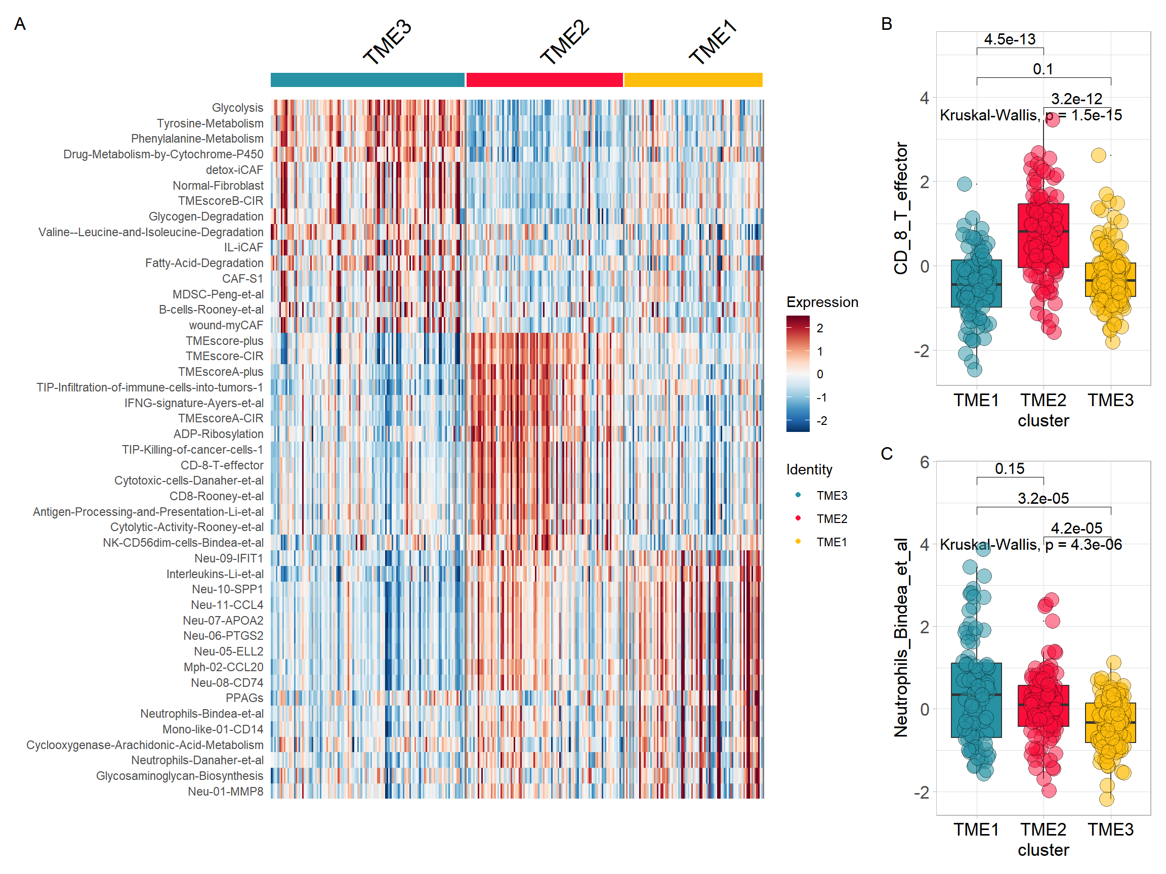
Survival differences between tumour microenvironment subtypes
## Loading required package: ggpubr## ℹ Loading cached data: "pdata_acrg"input <- merge(pdata_acrg, input, by = "ID")
p1 <- surv_group(
input_pdata = input,
target_group = "cluster",
ID = "ID",
reference_group = "High",
project = "ACRG",
cols = cols,
time = "OS_time",
status = "OS_status",
time_type = "month",
save_path = "result"
)## ℹ Follow-up time ranges from 1 to 105.7 months## TME1 TME2 TME3
## 85 96 119## ℹ Maximum follow-up time is 105.7 months; divided into 6 sections## Registered S3 methods overwritten by 'ggpp':
## method from
## heightDetails.titleGrob ggplot2
## widthDetails.titleGrob ggplot2## Ignoring unknown labels:
## • colour : "Strata"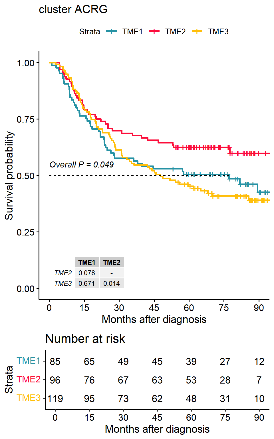
Relationship between tumour microenvironmental subtypes and other subtypes
## # A tibble: 12 × 5
## # Groups:   cluster [3]
##    cluster Subtype    Freq  Prop count
##    <chr>   <fct>     <dbl> <dbl> <dbl>
##  1 TME1    EMT          14  0.16    85
##  2 TME1    MSI          12  0.14    85
##  3 TME1    MSS/TP53-    34  0.4     85
##  4 TME1    MSS/TP53+    25  0.29    85
##  5 TME2    EMT           6  0.06    96
##  6 TME2    MSI          47  0.49    96
##  7 TME2    MSS/TP53-    22  0.23    96
##  8 TME2    MSS/TP53+    21  0.22    96
##  9 TME3    EMT          26  0.22   119
## 10 TME3    MSI           9  0.08   119
## 11 TME3    MSS/TP53-    51  0.43   119
## 12 TME3    MSS/TP53+    33  0.28   119
## [1] "'#374E55FF', '#DF8F44FF', '#00A1D5FF', '#B24745FF', '#79AF97FF', '#6A6599FF', '#80796BFF'"## # A tibble: 9 × 5
## # Groups: cluster [3]
## cluster Lauren Freq Prop count
## <chr> <fct> <dbl> <dbl> <dbl>
## 1 TME1 Diffuse 37 0.44 85
## 2 TME1 Intestinal 47 0.55 85
## 3 TME1 Mixed 1 0.01 85
## 4 TME2 Diffuse 31 0.32 96
## 5 TME2 Intestinal 54 0.56 96
## 6 TME2 Mixed 11 0.11 96
## 7 TME3 Diffuse 67 0.56 119
## 8 TME3 Intestinal 45 0.38 119
## 9 TME3 Mixed 7 0.06 119## [1] "'#374E55FF', '#DF8F44FF', '#00A1D5FF', '#B24745FF', '#79AF97FF', '#6A6599FF', '#80796BFF'"p3 <- percent_bar_plot(input, x = "cluster", y = "TMEscore_binary", palette = "jama", axis_angle = 60)## # A tibble: 7 × 5
## # Groups: cluster [3]
## cluster TMEscore_binary Freq Prop count
## <chr> <fct> <dbl> <dbl> <dbl>
## 1 TME1 High 5 0.06 85
## 2 TME1 Low 79 0.93 85
## 3 TME1 <NA> 1 0.01 85
## 4 TME2 High 59 0.61 96
## 5 TME2 Low 37 0.39 96
## 6 TME3 High 7 0.06 119
## 7 TME3 Low 112 0.94 119## [1] "'#374E55FF', '#DF8F44FF', '#00A1D5FF', '#B24745FF', '#79AF97FF', '#6A6599FF', '#80796BFF'"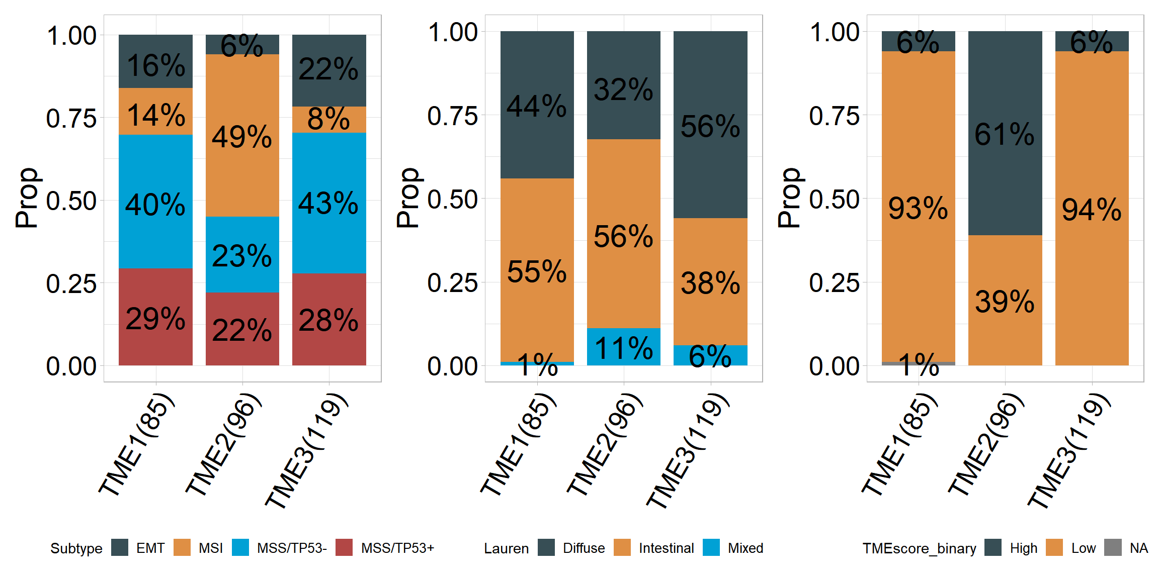
7.10 References
Cristescu, R., Lee, J., Nebozhyn, M. et al. Molecular analysis of gastric cancer identifies subtypes associated with distinct clinical outcomes. Nat Med 21, 449–456 (2015). https://doi.org/10.1038/nm.3850
CIBERSORT; Newman, A. M., Liu, C. L., Green, M. R., Gentles, A. J., Feng, W., Xu, Y., … Alizadeh, A. A. (2015). Robust enumeration of cell subsets from tissue expression profiles. Nature Methods, 12(5), 453–457. https://doi.org/10.1038/nmeth.3337;
Seurat: Hao and Hao et al. Integrated analysis of multimodal single-cell data. Cell (2021)
easier; Lapuente-Santana, Ó., van Genderen, M., Hilbers, P., Finotello, F., & Eduati, F. (2021). ‘Interpretable systems biomarkers predict response to immune-checkpoint inhibitors.’ Patterns (New York, N.Y.), 2(8), 100293.