Chapter 5 TME deconvolution
This section demonstrates various algorithms for parsing the tumour microenvironment using data from the bulk transcriptome. We also describe how to construct the reference signature matrix for the popular SVR algorithm (CIBERSORT) from single-cell data.
5.2 Downloading data for example
Obtaining data set from GEO Gastric cancer: GSE62254 using GEOquery R package.
if (!requireNamespace("GEOquery", quietly = TRUE)) BiocManager::install("GEOquery")
library("GEOquery")
# NOTE: This process may take a few minutes which depends on the internet connection speed. Please wait for its completion.
eset_geo <- getGEO(GEO = "GSE62254", getGPL = F, destdir = "./")
eset <- eset_geo[[1]]
eset <- exprs(eset)
eset[1:5, 1:5]
## GSM1523727 GSM1523728 GSM1523729 GSM1523744 GSM1523745
## 1007_s_at 3.2176645 3.0624323 3.0279131 2.921683 2.8456013
## 1053_at 2.4050109 2.4394879 2.2442708 2.345916 2.4328582
## 117_at 1.4933412 1.8067380 1.5959665 1.839822 1.8326058
## 121_at 2.1965561 2.2812181 2.1865556 2.258599 2.1874363
## 1255_g_at 0.8698382 0.9502466 0.8125414 1.012860 0.9441993Annotation of genes in the expression matrix and removal of duplicate genes.
library(IOBR)

# Load the annotation file `anno_hug133plus2` in IOBR.
anno_hug133plus2 <- load_data("anno_hug133plus2")
head(anno_hug133plus2)
## # A tibble: 6 × 2
## probe_id symbol
## <fct> <fct>
## 1 1007_s_at MIR4640
## 2 1053_at RFC2
## 3 117_at HSPA6
## 4 121_at PAX8
## 5 1255_g_at GUCA1A
## 6 1294_at MIR5193# Conduct gene annotation using `anno_hug133plus2` file; If identical gene symbols exists, these genes would be ordered by the mean expression levels. The gene symbol with highest mean expression level is selected and remove others.
eset <- anno_eset(
eset = eset,
annotation = anno_hug133plus2,
symbol = "symbol",
probe = "probe_id",
method = "mean"
)
eset[1:5, 1:3]## GSM1523727 GSM1523728 GSM1523729
## SH3KBP1 4.327974 4.316195 4.351425
## RPL41 4.246149 4.246808 4.257940
## EEF1A1 4.293762 4.291038 4.262199
## COX2 4.250288 4.283714 4.270508
## LOC101928826 4.219303 4.219670 4.2132525.3 Available Methods to Decode TME Contexture
## MCPcounter EPIC xCell CIBERSORT
## "mcpcounter" "epic" "xcell" "cibersort"
## CIBERSORT Absolute IPS ESTIMATE SVR
## "cibersort_abs" "ips" "estimate" "svr"
## lsei TIMER quanTIseq
## "lsei" "timer" "quantiseq"The input data is a matrix subseted from ESET of ACRG cohort, with genes in rows and samples in columns. The row name must be HGNC symbols and the column name must be sample names.
##              GSM1523727 GSM1523728 GSM1523729
## SH3KBP1        4.327974   4.316195   4.351425
## RPL41          4.246149   4.246808   4.257940
## EEF1A1         4.293762   4.291038   4.262199
## COX2           4.250288   4.283714   4.270508
## LOC101928826 4.219303 4.219670 4.213252Check detail parameters of the function
5.4 Method 1: CIBERSORT
## Warning: Data values appear small (< 50).
## ℹ Input should be in TPM/FPKM scale, not log-transformed
## ℹ Running CIBERSORT## ℹ Loading cached data: "lm22"# head(cibersort)
res <- cell_bar_plot(input = cibersort[1:12, ], features = colnames(cibersort)[3:24], title = "CIBERSORT Cell Fraction")## ℹ Available categories: box, continue2, continue, random, heatmap, heatmap3, tidyheatmap## ℹ Random palettes: 1 (palette1), 2 (palette2), 3 (palette3), 4 (palette4)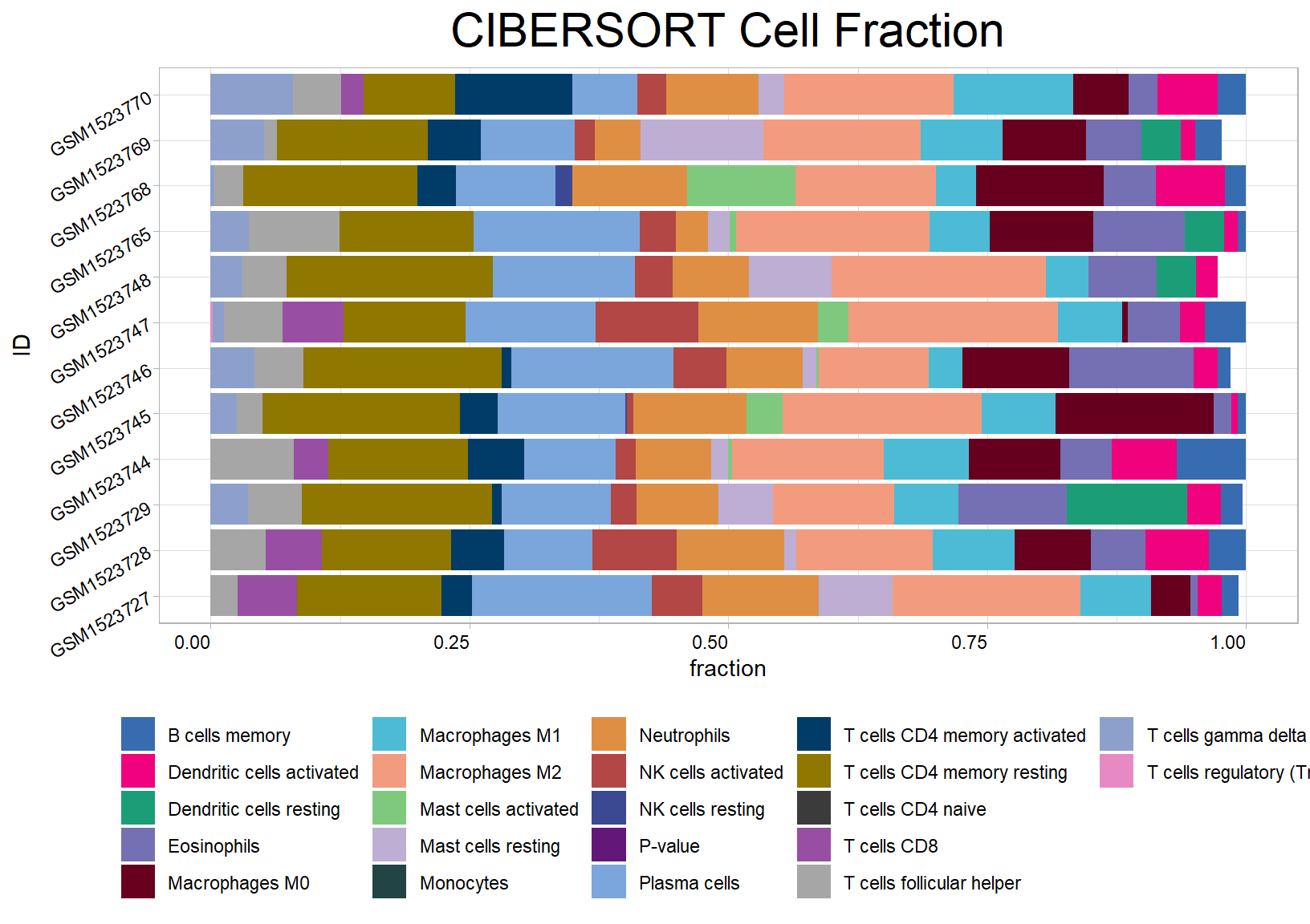
5.5 Method 2: EPIC
## Warning: Data values appear small (< 50).
## ℹ Input should be in TPM/FPKM scale, not log-transformed
## ℹ Running EPIC deconvolution## ℹ Loading cached data: "TRef"## ℹ Loading cached data: "mRNA_cell_default"## Warning in EPIC(bulk = eset, reference = ref, mRNA_cell = NULL, scaleExprs = TRUE): The optimization didn't fully converge for some samples:
## GSM1523744; GSM1523746; GSM1523781; GSM1523786
## - check fit.gof for the convergeCode and convergeMessage## Warning in EPIC(bulk = eset, reference = ref, mRNA_cell = NULL, scaleExprs =
## TRUE): mRNA_cell value unknown for some cell types: CAFs, Endothelial - using
## the default value of 0.4 for these but this might bias the true cell
## proportions from all cell types.## # A tibble: 6 × 9
## ID Bcells_EPIC CAFs_EPIC CD4_Tcells_EPIC CD8_Tcells_EPIC Endothelial_EPIC
## <chr> <dbl> <dbl> <dbl> <dbl> <dbl>
## 1 GSM152… 0.0292 0.00888 0.145 0.0756 0.0876
## 2 GSM152… 0.0293 0.0109 0.159 0.0745 0.0954
## 3 GSM152… 0.0308 0.0106 0.149 0.0732 0.0941
## 4 GSM152… 0.0273 0.0108 0.145 0.0704 0.0860
## 5 GSM152… 0.0280 0.0111 0.151 0.0707 0.0928
## 6 GSM152… 0.0320 0.00958 0.148 0.0716 0.0907
## # ℹ 3 more variables: Macrophages_EPIC <dbl>, NKcells_EPIC <dbl>,
## # otherCells_EPIC <dbl>5.6 Method 3: MCPcounter
## Warning: Data values appear small (< 50).
## ℹ Input should be in TPM/FPKM scale, not log-transformed
## ℹ Running MCP-counter deconvolution## # A tibble: 6 × 11
## ID T_cells_MCPcounter CD8_T_cells_MCPcounter Cytotoxic_lymphocytes_M…¹
## <chr> <dbl> <dbl> <dbl>
## 1 GSM1523727 1.47 1.11 1.33
## 2 GSM1523728 1.53 1.05 1.60
## 3 GSM1523729 1.47 1.07 1.37
## 4 GSM1523744 1.46 1.02 1.44
## 5 GSM1523745 1.51 1.10 1.49
## 6 GSM1523746 1.51 0.992 1.40
## # ℹ abbreviated name: ¹Cytotoxic_lymphocytes_MCPcounter
## # ℹ 7 more variables: B_lineage_MCPcounter <dbl>, NK_cells_MCPcounter <dbl>,
## # Monocytic_lineage_MCPcounter <dbl>,
## # Myeloid_dendritic_cells_MCPcounter <dbl>, Neutrophils_MCPcounter <dbl>,
## # Endothelial_cells_MCPcounter <dbl>, Fibroblasts_MCPcounter <dbl>5.7 Method 4: xCELL
## # A tibble: 6 × 68
##   ID         aDC_xCell Adipocytes_xCell Astrocytes_xCell `B-cells_xCell`
##   <chr>          <dbl>            <dbl>            <dbl>           <dbl>
## 1 GSM1523727 0                 0.000346         1.63e-21       0.0000410
## 2 GSM1523728 0.000221          0.000255         0              0.0000489
## 3 GSM1523729 0.0000141         0.000490         7.55e-20       0
## 4 GSM1523744 0.000110          0.000395         1.20e-20       0.0000600
## 5 GSM1523745 0.000100          0.000259         0              0.0000239
## 6 GSM1523746 0.0000415         0.000266         6.62e-20       0.0000637
## # ℹ 63 more variables: Basophils_xCell <dbl>,
## #   `CD4+_memory_T-cells_xCell` <dbl>, `CD4+_naive_T-cells_xCell` <dbl>,
## #   `CD4+_T-cells_xCell` <dbl>, `CD4+_Tcm_xCell` <dbl>, `CD4+_Tem_xCell` <dbl>,
## #   `CD8+_naive_T-cells_xCell` <dbl>, `CD8+_T-cells_xCell` <dbl>,
## #   `CD8+_Tcm_xCell` <dbl>, `CD8+_Tem_xCell` <dbl>, cDC_xCell <dbl>,
## #   Chondrocytes_xCell <dbl>, `Class-switched_memory_B-cells_xCell` <dbl>,
## #   CLP_xCell <dbl>, CMP_xCell <dbl>, DC_xCell <dbl>, …
5.8 Method 5: ESTIMATE
## [1] "Merged dataset includes 9940 genes (472 mismatched)."## [1] "1 gene set: StromalSignature overlap= 136"
## [1] "2 gene set: ImmuneSignature overlap= 138"## # A tibble: 6 × 5
## ID StromalScore_estimate ImmuneScore_estimate ESTIMATEScore_estimate
## <chr> <dbl> <dbl> <dbl>
## 1 GSM1523727 -1250. 268. -982.
## 2 GSM1523728 197. 1334. 1531.
## 3 GSM1523729 -111. 822. 711.
## 4 GSM1523744 -119. 662. 544.
## 5 GSM1523745 324. 1015. 1339.
## 6 GSM1523746 -594. 621. 27.0
## # ℹ 1 more variable: TumorPurity_estimate <dbl>5.9 Method 6: TIMER
timer <- deconvo_tme(eset = eset_acrg, method = "timer", group_list = rep("stad", dim(eset_acrg)[2]))
head(timer)
## # A tibble: 6 × 7
## ID B_cell_TIMER T_cell_CD4_TIMER T_cell_CD8_TIMER Neutrophil_TIMER
## <chr> <dbl> <dbl> <dbl> <dbl>
## 1 GSM1523727 0.104 0.128 0.183 0.108
## 2 GSM1523728 0.103 0.130 0.192 0.118
## 3 GSM1523729 0.106 0.130 0.190 0.110
## 4 GSM1523744 0.101 0.126 0.187 0.111
## 5 GSM1523745 0.104 0.127 0.191 0.116
## 6 GSM1523746 0.105 0.129 0.192 0.111
## # ℹ 2 more variables: Macrophage_TIMER <dbl>, DC_TIMER <dbl>5.10 Method 7: quanTIseq
quantiseq <- deconvo_tme(eset = eset_acrg, tumor = TRUE, arrays = TRUE, scale_mrna = TRUE, method = "quantiseq")## Warning: Data values appear small (< 50).
## ℹ Input should be in TPM/FPKM scale, not log-transformed## ℹ Running quanTIseq deconvolution## ℹ Running quanTIseq deconvolution module## ℹ Loading cached data: "quantiseq_data"## ℹ Gene expression normalization and re-annotation (arrays: TRUE)## ℹ Loading cached data: "quantiseq_data"## ℹ Removing 17 genes with high expression in tumors## ℹ Signature genes found in data set: 152/153 (99.35%)## ℹ Mixture deconvolution (method: lsei)## ✔ Deconvolution successful!## # A tibble: 6 × 12
## ID B_cells_quantiseq Macrophages_M1_quantiseq Macrophages_M2_quantiseq
## <chr> <dbl> <dbl> <dbl>
## 1 GSM1523727 0.0983 0.0510 0.0598
## 2 GSM1523728 0.0967 0.0795 0.0607
## 3 GSM1523729 0.102 0.0450 0.0758
## 4 GSM1523744 0.0954 0.0725 0.0579
## 5 GSM1523745 0.0991 0.0669 0.0613
## 6 GSM1523746 0.105 0.0453 0.0662
## # ℹ 8 more variables: Monocytes_quantiseq <dbl>, Neutrophils_quantiseq <dbl>,
## # NK_cells_quantiseq <dbl>, T_cells_CD4_quantiseq <dbl>,
## # T_cells_CD8_quantiseq <dbl>, Tregs_quantiseq <dbl>,
## # Dendritic_cells_quantiseq <dbl>, Other_quantiseq <dbl>res <- cell_bar_plot(input = quantiseq[1:12, ], id = "ID", features = colnames(quantiseq)[2:12], title = "quanTIseq Cell Fraction")## ℹ Available categories: box, continue2, continue, random, heatmap, heatmap3, tidyheatmap## ℹ Random palettes: 1 (palette1), 2 (palette2), 3 (palette3), 4 (palette4)5.11 Method 8: IPS
## # A tibble: 6 × 7
##   ID         MHC_IPS EC_IPS SC_IPS  CP_IPS AZ_IPS IPS_IPS
##   <chr>        <dbl>  <dbl>  <dbl>   <dbl>  <dbl>   <dbl>
## 1 GSM1523727    2.25  0.404 -0.192  0.220    2.68       9
## 2 GSM1523728    2.37  0.608 -0.578 -0.234    2.17       7
## 3 GSM1523729    2.10  0.480 -0.322  0.0993   2.36       8
## 4 GSM1523744    2.12  0.535 -0.333  0.0132   2.34       8
## 5 GSM1523745    1.91  0.559 -0.479  0.0880   2.08       7
## 6 GSM1523746    1.94  0.458 -0.346  0.261    2.31       8
5.12 Combination of above deconvolution results
tme_combine <- cibersort %>%
  inner_join(., mcp, by = "ID") %>%
  inner_join(., xcell, by = "ID") %>%
  inner_join(., epic, by = "ID") %>%
  inner_join(., estimate, by = "ID") %>%
  inner_join(., timer, by = "ID") %>%
  inner_join(., quantiseq, by = "ID") %>%
  inner_join(., ips, by = "ID")
dim(tme_combine)
## [1] 50 1385.13 How to customise the signature matrix for SVR and lesi algorithm
The recent surge in single-cell RNA sequencing has enabled us to identify novel microenvironmental cells, tumour microenvironmental characteristics, and tumour clonal signatures with high resolution. It is necessary to scrutinize, confirm and depict these features attained from high-dimensional single-cell information in bulk-seq with extended specimen sizes for clinical phenotyping. This is a demonstration using the results of 10X single-cell sequencing data of PBMC to construct gene signature matrix for deconvo_tme function and estimate the abundance of these cell types in bulk transcriptome data.
Download PBMC dataset through: https://cf.10xgenomics.com/samples/cell/pbmc3k/pbmc3k_filtered_gene_bc_matrices.tar.gz
Initialize the Seurat object with the raw (non-normalized data).
library(Seurat)
pbmc.data <- Read10X(data.dir = "./pbmc3k_filtered_gene_bc_matrices/filtered_gene_bc_matrices/hg19")
pbmc <- CreateSeuratObject(counts = pbmc.data, project = "pbmc3k", min.cells = 3, min.features = 200)
Data prepare using Seurat’s standard pipeline.
pbmc <- FindVariableFeatures(pbmc, selection.method = "vst", nfeatures = 2000, verbose = FALSE)
pbmc <- NormalizeData(pbmc, normalization.method = "LogNormalize", scale.factor = 10000, verbose = FALSE)
pbmc <- ScaleData(pbmc, features = rownames(pbmc), verbose = FALSE)
pbmc <- RunPCA(pbmc, features = VariableFeatures(object = pbmc), verbose = FALSE)
pbmc <- FindNeighbors(pbmc, dims = 1:10, verbose = FALSE)
pbmc <- FindClusters(pbmc, resolution = 0.5, verbose = FALSE)
# Annotate cells according to seurat's tutorials
# https://satijalab.org/seurat/articles/pbmc3k_tutorial
new.cluster.ids <- c("Naive_CD4_T", "CD14_Mono", "Memory_CD4_T", "Bcells", "CD8_Tcell", "FCGR3A_Mono", "NK", "DC", "Platelet")
names(new.cluster.ids) <- levels(pbmc$seurat_clusters)
pbmc <- RenameIdents(pbmc, new.cluster.ids)
pbmc$celltype <- Idents(pbmc)
Generate reference matrix using generateRef_seurat function.
##
##       Bcells    CD14_Mono    CD8_Tcell           DC  FCGR3A_Mono Memory_CD4_T
##          349          491          339           36          159          467
##  Naive_CD4_T           NK     Platelet
##          696          148           15
## p_val avg_log2FC pct.1 pct.2 p_val_adj cluster gene
## RPS6 5.433910e-142 0.6874852 0.999 0.994 7.452065e-138 Naive_CD4_T RPS6
## RPL32 5.645212e-138 0.6331843 0.999 0.995 7.741843e-134 Naive_CD4_T RPL32
## RPS12 5.615968e-137 0.7246307 1.000 0.990 7.701739e-133 Naive_CD4_T RPS12
## RPS27 1.903184e-131 0.7039172 0.999 0.992 2.610026e-127 Naive_CD4_T RPS27
## RPS25 2.355892e-127 0.7846319 0.997 0.973 3.230871e-123 Naive_CD4_T RPS25
## RPL31 3.961343e-121 0.7725688 0.996 0.963 5.432585e-117 Naive_CD4_T RPL31
## # A tibble: 450 × 7
## # Groups: cluster [9]
## p_val avg_log2FC pct.1 pct.2 p_val_adj cluster gene
## <dbl> <dbl> <dbl> <dbl> <dbl> <fct> <chr>
## 1 5.43e-142 0.687 0.999 0.994 7.45e-138 Naive_CD4_T RPS6
## 2 5.62e-137 0.725 1 0.99 7.70e-133 Naive_CD4_T RPS12
## 3 1.90e-131 0.704 0.999 0.992 2.61e-127 Naive_CD4_T RPS27
## 4 2.36e-127 0.785 0.997 0.973 3.23e-123 Naive_CD4_T RPS25
## 5 3.96e-121 0.773 0.996 0.963 5.43e-117 Naive_CD4_T RPL31
## 6 1.74e-113 0.743 0.996 0.969 2.38e-109 Naive_CD4_T RPL9
## 7 1.08e-104 0.779 0.996 0.974 1.48e-100 Naive_CD4_T RPS3A
## 8 3.04e-104 1.11 0.895 0.592 4.16e-100 Naive_CD4_T LDHB
## 9 8.09e-101 0.749 0.996 0.964 1.11e- 96 Naive_CD4_T RPS27A
## 10 5.99e- 90 0.688 0.986 0.956 8.22e- 86 Naive_CD4_T RPS13
## # ℹ 440 more rowsLoad the bulk RNA-seq data
eset_stad <- load_data("eset_stad")
eset <- count2tpm(countMat = eset_stad, source = "local", idType = "ensembl")
svr <- deconvo_tme(eset = eset, reference = sm, method = "svr", arrays = FALSE, absolute.mode = FALSE, perm = 100)
head(svr)
## # A tibble: 6 × 13
## ID Naive-CD4-T_CIBERSOR…¹ `CD14-Mono_CIBERSORT` Memory-CD4-T_CIBERSO…²
## <chr> <dbl> <dbl> <dbl>
## 1 TCGA-BR-6… 0.0935 0.0273 0
## 2 TCGA-BR-7… 0 0.00796 0.0897
## 3 TCGA-BR-8… 0.117 0 0
## 4 TCGA-BR-8… 0.200 0 0
## 5 TCGA-BR-8… 0.115 0 0
## 6 TCGA-BR-8… 0 0.00258 0.0681
## # ℹ abbreviated names: ¹`Naive-CD4-T_CIBERSORT`, ²`Memory-CD4-T_CIBERSORT`
## # ℹ 9 more variables: Bcells_CIBERSORT <dbl>, `CD8-Tcell_CIBERSORT` <dbl>,
## # `FCGR3A-Mono_CIBERSORT` <dbl>, NK_CIBERSORT <dbl>, DC_CIBERSORT <dbl>,
## # Platelet_CIBERSORT <dbl>, `P-value_CIBERSORT` <dbl>,
## # Correlation_CIBERSORT <dbl>, RMSE_CIBERSORT <dbl>5.14 References
If you use this package in your work, please cite both our package and the method(s) you are using.
Citation and licenses of these deconvolution methods
CIBERSORT; free for non-commerical use only; Newman, A. M., Liu, C. L., Green, M. R., Gentles, A. J., Feng, W., Xu, Y., … Alizadeh, A. A. (2015). Robust enumeration of cell subsets from tissue expression profiles. Nature Methods, 12(5), 453–457. https://doi.org/10.1038/nmeth.3337;
ESTIMATE; free (GPL2.0); Vegesna R, Kim H, Torres-Garcia W, …, Verhaak R. (2013). Inferring tumour purity and stromal and immune cell admixture from expression data. Nature Communications 4, 2612. http://doi.org/10.1038/ncomms3612;
quanTIseq; free (BSD); Finotello, F., Mayer, C., Plattner, C., Laschober, G., Rieder, D., Hackl, H., …, Sopper, S. (2019). Molecular and pharmacological modulators of the tumor immune contexture revealed by deconvolution of RNA-seq data. Genome medicine, 11(1), 34. https://doi.org/10.1186/s13073-019-0638-6;
TIMER; free (GPL 2.0); Li, B., Severson, E., Pignon, J.-C., Zhao, H., Li, T., Novak, J., … Liu, X. S. (2016). Comprehensive analyses of tumor immunity: implications for cancer immunotherapy. Genome Biology, 17(1), 174. https://doi.org/10.1186/s13059-016-1028-7;
IPS; free (BSD); P. Charoentong et al., Pan-cancer Immunogenomic Analyses Reveal Genotype-Immunophenotype Relationships and Predictors of Response to Checkpoint Blockade. Cell Reports 18, 248-262 (2017). https://doi.org/10.1016/j.celrep.2016.12.019;
MCPCounter; free (GPL 3.0); Becht, E., Giraldo, N. A., Lacroix, L., Buttard, B., Elarouci, N., Petitprez, F., … de Reyniès, A. (2016). Estimating the population abundance of tissue-infiltrating immune and stromal cell populations using gene expression. Genome Biology, 17(1), 218. https://doi.org/10.1186/s13059-016-1070-5;
xCell; free (GPL 3.0); Aran, D., Hu, Z., & Butte, A. J. (2017). xCell: digitally portraying the tissue cellular heterogeneity landscape. Genome Biology, 18(1), 220. https://doi.org/10.1186/s13059-017-1349-1;
EPIC; free for non-commercial use only (Academic License); Racle, J., de Jonge, K., Baumgaertner, P., Speiser, D. E., & Gfeller, D. (2017). Simultaneous enumeration of cancer and immune cell types from bulk tumor gene expression data. ELife, 6, e26476. https://doi.org/10.7554/eLife.26476;
GSVA free (GPL (>= 2)) Hänzelmann S, Castelo R, Guinney J (2013). “GSVA: gene set variation analysis for microarray and RNA-Seq data.” BMC Bioinformatics, 14, 7. doi: 10.1186/1471-2105-14-7, http://www.biomedcentral.com/1471-2105/14/7